


1 INTRODUCTION
The Korean Pathfinder Lunar Orbiter (KPLO) is lunar exploration mission expected to launch after 2018 with an orbit about 100 km above the surface of the Moon. The Korea Aerospace Research Institute (KARI) is currently developing an entire system including the space, launch and ground segments. The ground segment consists of two centers, the mission operation center (MOC) and the payload data center (PDC). The MOC consists of subsystems such as the telemetry, tracking and command (TTC) subsystem, the real-time operation subsystem (ROS) and the flight dynamic subsystem (FDS) (Song et al. 2016). The Yonsei University has been participating in the development of the FDS, and has generated a prototype orbit determination software (Lee et al. 2016). The deep space orbit determination software (DSODS) is an improved form of the prototype software, which was developed using a MATLAB based Object Oriented Programming scheme and comprises of several submodules, i.e., orbit determination (OD), orbit prediction (OP), data simulation (DS) and event prediction (EP) (Kim et al. 2017).
Various orbit determination softwares were employed in previous deep space missions. The SMART-1 mission used Advanced Modular Facility for Interplanetary Navigation (AMFIN) libraries (Mackenzie et al. 2004). The GEODYN was used for precise orbit determination in the case of the Chang’e-1, the first Chinese lunar exploration mission (Jianguo et al. 2010), and the Lunar Reconnaissance Orbiter (LRO) which provided a high-resolution survey of the Moon (Mazarico et al. 2012). For the Lunar Atmosphere and Dust Environment Explorer (LADEE) mission, that aimed at determining the composition of the lunar atmosphere, dust environment and viability of optical laser communication technologies (D’Ortenzio et al. 2015), the orbit determination tool kit (ODTK), a commercial software of the AGI, was used for the operation. Although commercial softwares are verified through various missions and are easy to use, they are hard to maintain and improve since their internal source codes are not provided. The DSODS is an independent software developed to support the KPLO, and serves as an asset of Korean space exploration. Moreover, it can be extended to the other deep space missions in the future.
The objectives of this research are to develop, demonstrate and validate DSODS. For the demonstration and validation, tracking data from the Lunar Prospector, provided by the NASA planetary data system (PDS), was applied to the DSODS. A Monte-Carlo simulation is conducted to verify the statistical correlation between orbit solutions and the estimated covariance matrix. Furthermore, the results are analyzed through solution comparison and overlap analysis. Section 2 presents the construction of DSODS and some details of the sub-modules, such as the functionality requirements and subroutines. The demonstration and validation of results using the Lunar Prospector tracking data, are described in Sections 3 and 4, respectively. Section 5 summarizes the overall results.
2 ORBIT DETERMINATION SOFTWARE
The current orbit determination software is designed and developed to satisfy the orbit determination requirement of the KPLO. Since a quantitative requirement has not yet been established, the software is aimed at acquiring an orbital accuracy of 1 km, identical to that on the existing lunar exploration mission, Lunar Prospector (Binder et al. 1998). This section addresses the overall construction and details of the DSODS.
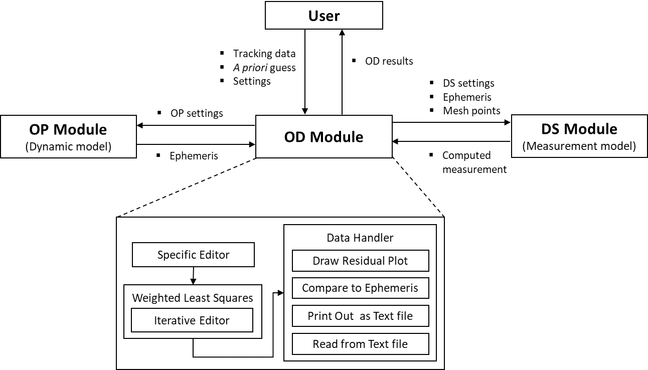
Orbit determination is procedure to obtain parameters that are related to the motion and the tracking data of the spacecraft. The procedure requires a system model and an estimation algorithm to predict the tracking data and estimate parameters using actual tracking data. The system model can be divided into a dynamic model and a measurement model. The dynamic model includes the force models acting on the spacecraft and a numerical integrator for the orbit propagation. The measurement model includes the tracking algorithm and hardware characteristics to simulate the tracking data. In the DSODS, each model is implemented in two submodules: OP module and DS module. Furthermore, the OD module consists of an estimation algorithm and some useful subroutines. Kim et al. (2017) presented an overview of the DSODS, including its construction, data flow and user interfaces of the submodules. Fig. 1 shows the brief data flow of DSODS and subroutines of the module, whose details are explained subsequently.
In case of the OP module, a general mission analysis tool (GMAT) is employed as a third-party software component using a MATLAB-executable (MEX) interface (Kim et al. 2017). The GMAT was developed by NASA GSFC and has been used in missions such as the Lunar Crater Observation and Sensing Satellite (LCROSS) and the Acceleration, Reconnection, Turbulence and Electrodynamics of the Moon’s Interaction with the Sun (ARTEMIS). The force model and numerical integrator (propagator) are determined and validated using multiple test scripts (Hughes et al. 2014). The OP module receives the settings for the orbital prediction, such as a gravity model and accuracy of the propagator, from the OD module, and transfers the propagated states set, i.e., ephemeris, in the form of a satellite tool kit (STK) format.
Alternatively, the DS module is developed by Yonsei to simulate the tracking data. NASA’s deep space network (DSN), near earth network (NEN) and universal space network (USN) are usually employed for deep space missions (Policastri et al. 2015), and these stations provide various types of tracking data such as tracking angles, un-ramped two-way range and Doppler, and the difference between the uplink and the downlink frequency divided by the transponding ratio of the spacecraft (Chang 2015). In the DSODS, un-ramped two-way range and Doppler are modeled by the DS module, where the corrections for tropospheric delay and antenna offset delay are involved. I should be noted that the ramped range and Doppler, and the corrections for ionospheric delay and charged particle delay are being developed and will be added to the DS module. The DS module simulates tracking data by utilizing the configuration for the DS, the ephemeris and the mesh points are transferred from OD module, and the simulated tracking data is returned to the OD module.
In the OD module, a batch least squares algorithm is implemented. The batch type estimation is a post-processing method that treats all the observed data of an arc to determine the states at a specific epoch, while the sequential estimation algorithm estimates the states sequentially at each observation time. Batch estimation is a simple, more accurate and robust technique compared to sequential estimation algorithms, like the Kalman filter (Crassidis & Junkins 2011). The functionality requirements and subroutine algorithms are addressed in the following sections.
The OD module is required to provide some necessary range of operations. Table 1 presents the functionality requirements of the OD module (Song et al. 2016). The functionality code categorizes the functionality requirement, and can consist of some sub-codes. In case of the ODF-0 (to read and write information from/to a text file), for instance, there are two sub-codes to print out and load information, and each function is developed within the OD module. Note that the functionality requirements and the correlated codes are subject to change should the details of the mission requirement and operating concepts change.
The OD module consists of multiple subroutines to estimate parameters, improve performance and support additional analysis. In this section, some representative subroutines, the weighted batch least squares, the specific/iterative data editor and the data handler are briefly explained.
The batch least squares algorithm estimates parameters using a system model (F):(1)
In case of the OD, Y is the tracking data, є is the measurement error vector, and X is a ‘solve-for’ vector, which is to be estimated such as the position or velocity vector (Schutz et al. 2004). The system model is usually composed of the dynamic model and the measurement model.
The estimation can be referred to as an optimization, which minimizes the performance index (I), weighted sum of the squares of the measurement residual and the difference from a priori states:(2)
where and X0 are the a priori covariance matrix and ‘solve-for’ vector, respectively, and W is the weight matrix. The a priori covariance matrix and weight matrix correspond to the a priori uncertainty and measurement noise:(3)
where σj is the standard deviation of the jth element of the ‘solve-for’ vector, n is the dimension of the ‘solve-for’ vector, ϱk is the noise level of the kth tracking data measurement and m is total number of tracking data measurements.
The optimal solution is evaluated by the Newton-Rapson method, that uses 1st order approximations under the assumption of differentiability of the system model and the suitability of the ca priori states. Through several iterations, the ‘solve-for’ vector is updated using the variate of the ith iteration (ΔXi) (Long et al. 1989):(4)
where H is the Jacobian matrix, a partial derivative of the system model, that is numerically evaluated by that central differencing method in the OD module.
The convergence criterion is the cost reduction ratio (γ):(5)
The estimation sequence stops if the ratio becomes less than a small tolerance (ε), set as 10-3 by default, and also terminates when the number of iterations reach a designated maximum number.
The covariance matrix (P), which corresponds to the precision of the estimation, is evaluated after convergence by the following expression:(6)
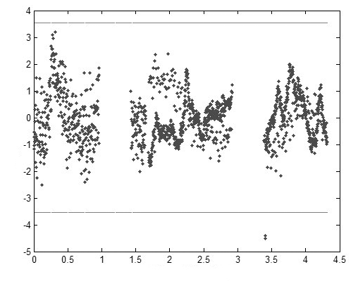
Data editing is done to reject any abnormal observation data that diminishes the accuracy of the solution from the orbit determination process. There are two types of data editors in the developed software. The first one is the specific editor, where the user designates a specific type, site and date of the observation. It is useful when the user has the empirical skills and when there are known problems with some observatories or dates. Another editor is the iterative editor, which is automatically executes every iteration. The iterative editor rejects the observation data if the data does not meet the conditions that are calculated by the measurement residuals and the states of the iteration (Long et al. 1989).(7)
In the above expression, wj is a weight component corresponding to the j-th observation data, yj is a j-th measurement residual, k is a constant multiplier and K is an additive constant. The predicted root mean square, PRMS, is evaluated by following form.(8)
Fig. 2 is an example of iterative editing using the weighted residual method, where two abnormal observation data points, which are circumscribed, are edited.
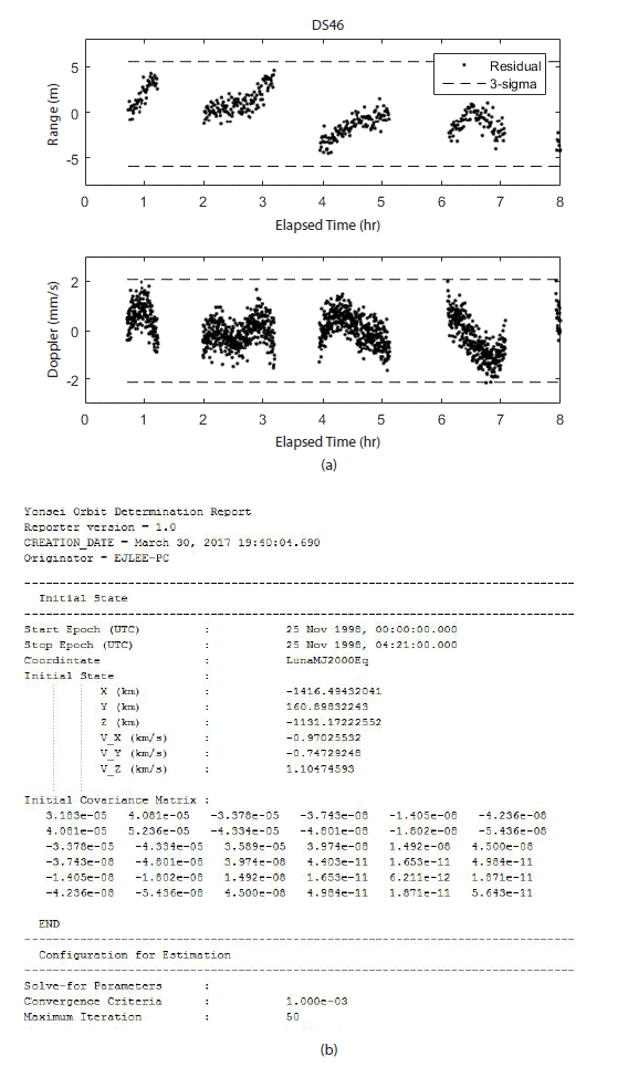
All information about the orbit determination including the dynamic model, tolerance, maximum iteration number and the estimated result are saved in the orbit determination data handler. The handler can generate a residual plot, compare the estimation results to the ephemeris and print the information to an ASCII file. The handler also can read the output file, load the configuration and the result from the file and utilize this information for the next orbit determination. Fig. 3 shows the residual plot and the output ASCII file.
3 DEMONSTRATION OF ROBUSTNESS
Software verification is a process to demonstrate that the program satisfies its requirement. There are various methods for verification such as mathematical analyses, reliability tests and process assurance (Sommerville 2011). In this section, a stress test, a test in an environment outside the normal operation limit, is conducted to demonstrate the robustness of the DSODS using Lunar Prospector tracking data. The Lunar Prospector was a lunar exploration mission to analyze the moon’s gravity and magnetic field, launched in 1998 (Binder 1998). The mission data is employed for the demonstration process as it orbited at an altitude of 100 km above the moon, just as the KPLO. Additionally, various datasets such as DSN tracking data, ephemeris and command log are available from the NASA PDS, which is an archive of data products from past NASA planetary missions.
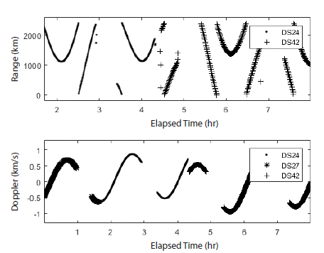
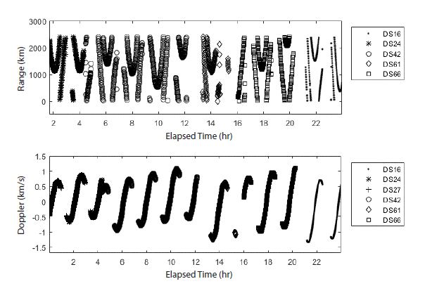
The orbit determination environment including the force model, the propagator options, the a priori covariance matrix and the weights for the measurement, is compiled in Table 2. The force model and the propagator are implemented in the GMAT, and the measurement weight is assigned based on the nominal noise level of the S-band tracking data (Chang 2015). The ‘solve-for’ parameters are threedimensional position and velocity vectors, and the range and Doppler biases of each tracking station. Fig. 4 shows the 8 hrs' tracking data, un-ramped two-way range and Doppler data provided by the 2 DSN stations, the DSS-24 (Goldstone, USA) and the DSS-42 (Canberra, Australia), also the DSS- 27 (Goldstone, USA) provides only the un-ramped two-way Doppler data. The NASA PDS1 ephemeris is considered as the true state, with an accuracy of approximately 1 km in position and 1 m/s in velocity2.
A set of a priori state vectors are generated by adding pseudo Gaussian errors to the true states, where the errors correspond to an a priori covariance matrix (Table 2). The a priori error is set as 1 km for position and 0.001 km/s for velocity, in accordance to the ephemeris accuracy of the Lunar Prospector. Note that the a priori error of biases are ignored, i.e., a priori biases are fixed as zero since the robustness is checked only for the position and velocity vector of the spacecraft. The orbit solutions are evaluated using the generated a priori states set of 20 state vectors, and are statistically analyzed.
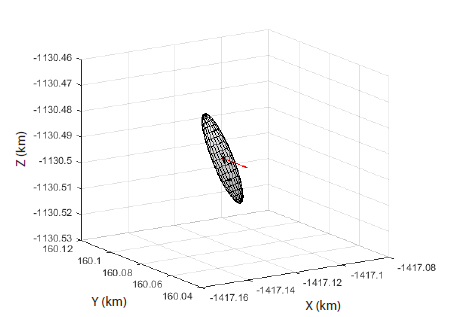
Fig. 5 shows the statistical covariance ellipsoid and the distribution of the solutions, where the major axis of the ellipsoid is normal to the direction towards the Earth. Since the tracking data, range and Doppler, is measured in the radial direction, uncertainty in the radial direction is much smaller than the along-track and cross-track directions. The solutions are distributed with a three-dimensional standard deviation of 18.66 m, which satisfies the mission requirement of the KPLO. The precision, however, is predicted as ~ 4 m by the estimated covariance matrix (as mentioned in Section 2.3), which includes the orbit solutions within a 5σ ellipsoid. Since the statistical consistence of the developed software has already been confirmed by that the estimated covariance matrix and the distribution of the actual solutions are consistent under the simplified environment (Lee et al. 2016), the causes that under-estimate the covariance matrix in comparison to the solution distribution in this study are analyzed considering the characteristics of the actual system. The first cause is the process noise, which denotes the unmodeled phenomena in the dynamic and measurement models. The covariance matrix evaluated by a batch type estimator does not contain process noise, but instead a a correlation matrix, which presents uncertainty of system-related parameters, ‘consider parameter’. The system model parameters, such as the geopotential coefficients and the solar radiation coefficients, can be used as the consider parameter, and their uncertainties can be modeled in the correlation matrix. In this analysis, however, no consider parameter is employed, resulting in an additional estimation error. The other cause is the inaccuracy of the a priori covariance and weight matrices. Since the uncertainty of a priori states and the noise level of the tracking data are not exactly determined, the covariance matrix has a corresponding error. Furthermore, the truncation error and round-off error also contribute to the estimation error.
Through the stress test, the robustness of the DSODS can be demonstrated within an a priori error margin of about 1 km. Moreover, the estimated covariance matrix can be regarded as an indicator of the precision of the orbit solution.
4 VALIDATION
The orbit determination software should provide an orbit solution to appropriately operate the mission. In this section, the accuracy of the DSODS is validated using Lunar Prospector tracking data and two types of analyses: (1) solution comparison to the NASA PDS ephemeris and (2) overlap analysis. Note that the tracking data and environment for validation are same as the demonstration procedure.
A comparison between solutions achieved through different systems is one of the methods to assess the accuracy of an orbit solution (Schutz et al. 2004). To confirm whether the developed software can prove suitably reliable for a mission, the orbit solution is evaluated using Lunar Prospector tracking data propagated over 24 hr, and is compared to the NASA PDS ephemeris.
In this study, an orbit determination is executed once in a day over the lunar orbit using one-day long tracking data, range and Doppler data, since the mission operation concept of the KPLO is not fixed yet. The arc length is 24 hr on November 25, 1998, using the tracking data provided by several DSN stations, as configured in Fig. 6. Un-ramped two-way range and Doppler data was provided by 5 DSN stations, DSS-16 in Goldstone, USA, and DSS-24, DSS-42, DSS-61 and DSS-66 in Madrid, Spain, with additional unramped two-way Doppler data supplied by a single DSN station, DSS-27 in Goldstone, USA.
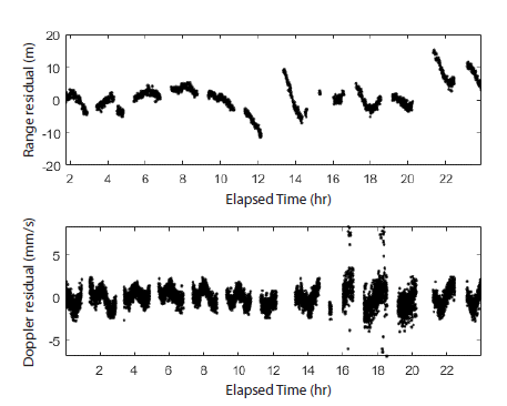
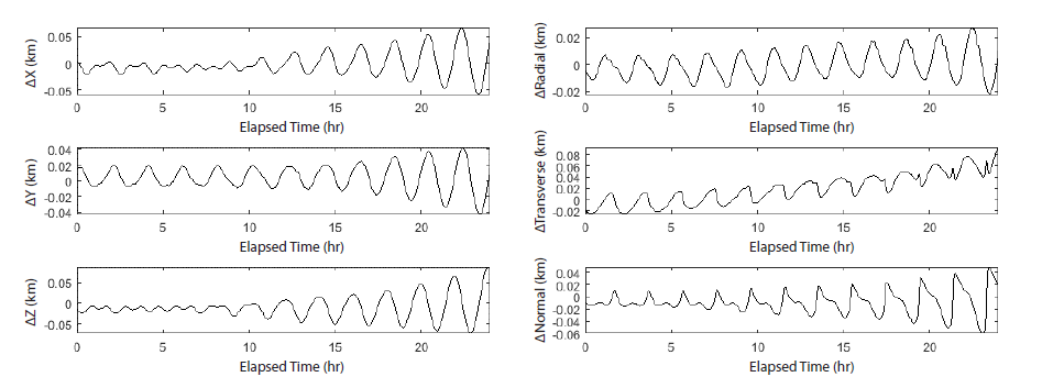
After the orbit determination, the standard deviations of the residuals are 4.28 m for range and 1.13 mm/s for Doppler, which correspond to the noise level of the S-band tracking data (Fig. 7). The system model however, should be improved since the residuals are not completely random distributions, i.e., include the existence of a systematic error. The position difference of the orbit solution with respect to the NASA PDS ephemeris is presented in Fig. 8. The variation by axis is conspicuous in the orbital frame, i.e., radial-transverse-normal frame, although not in the original inertial frame. The radial difference is the smallest, while the transverse-normal frame differences show an increase from 2 to 4 times after 24 hr. This is also due to the characteristics of the tracking system which measure the range and Doppler in the radial direction. Note that although the difference accumulates with time due to the nonlinearity of the dynamic system, the RMS of the difference over 24 hr is 39.51 m which is significantly lower than the orbit accuracy of the Lunar Prospector (1 km). Through solution comparison, the performance of the DSODS is deemed appropriate to support the KPLO.
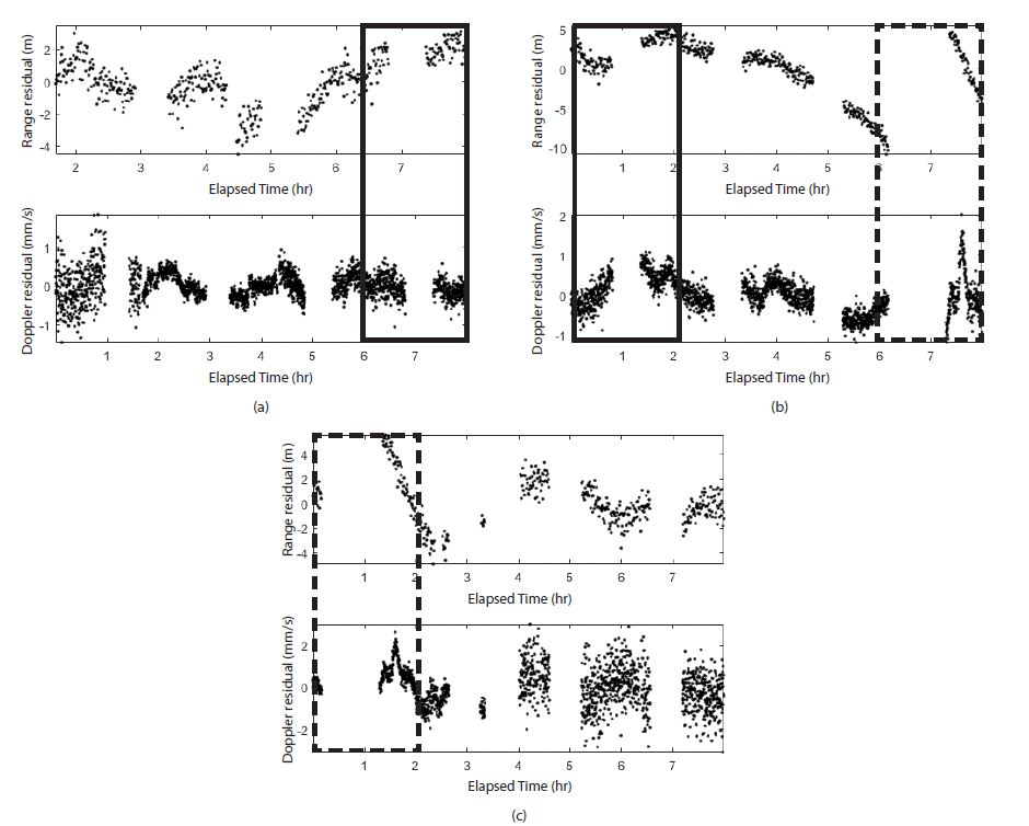
Overlapping is another technique to measure the accuracy of the orbit solution. The differences between separated arcs that share some part of tracking data are evaluated and considered indicators of orbit accuracy (Schutz et al. 2004). In this analysis, an 8 hrs' arc is designated and neighboring arcs are separated with 6 hrs' interval, that share 2 hr of tracking data. The tracking data used for the overlap analysis is the data of November 25, 1998, same as that used in the previous section.
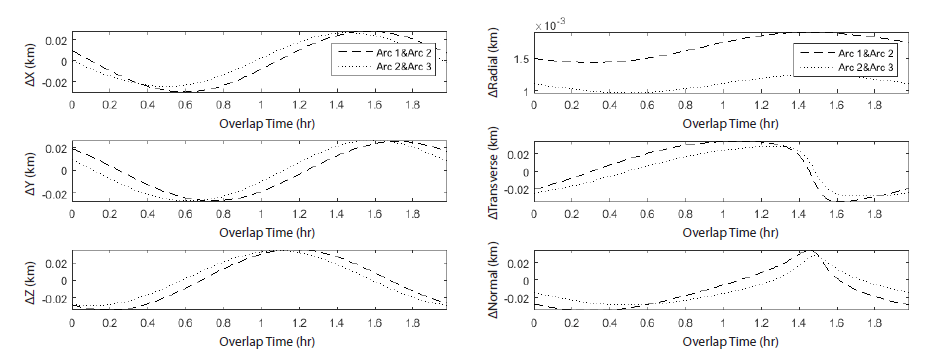
Fig. 9 shows the residuals of each arc, where two types of boxes, solid and dash, represent overlapped tracking data. The standard deviations of the range residuals are 1.40 m, 3.64 m and 1.93 m for each arc, and that of Doppler are 0.33 mm/s, 0.43 mm/s and 0.92 mm/s (Table 3). The residuals correspond to the nominal noise level of the S-band tracking data, signifying that the orbit solution is well converged by iterative process. However, the difference between the residuals of arcs is at least double due to a systematic error which needs further improvement. Fig. 10 is the position variation between the overlapped arcs with RMS position differences of 36.68 m and 50.14 m, with most differences concentrated in the transverse and normal directions. These differences correspond to the results from the previous section, confirming the consistency of the software and validating the accuracy of the DSODS to several tens of meters.
| Arc 1 | Arc 2 | Arc 3 | |
|---|---|---|---|
| Range (m) | 1.40 | 3.64 | 1.93 |
| Doppler (mm/s) | 0.33 | 0.43 | 0.92 |
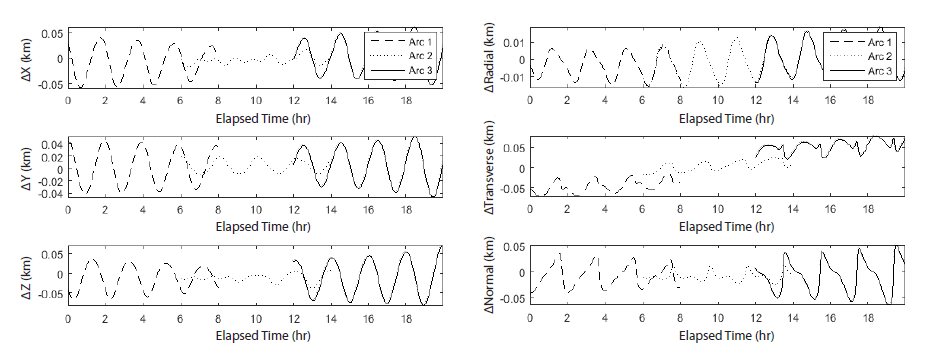
In addition, Fig. 11 presents the position difference of each arc compared to the NASA PDS ephemeris, with the RMS differences of 54.41 m, 20.23 and 63.55 m, respectively. These differences are also of the same order as the previous section. Here too the differences in the radial direction are minimum and almost same for all arcs, while those in the transversenormal directions have considerable variations between arcs. The discordance between the residual level and the position difference is interpreted as a systematic property caused by the shortage of information in the transverse and normal directions due to the characteristics of the tracking system.
5 SUMMARY
In this study, a DSODS is developed and is validated using Lunar Prospector tracking data. The DSODS consists of several submodules where the modules interact with each other. The OP module includes a force model and orbit propagator, that plays the role of a dynamic model in the orbit determination process. A GMAT is employed as an OP module for the DSODS. A DS module provides a DSN tracking data model, including hardware properties and some error sources. The OD module uses a batch type weighted least squares estimator for evaluation, and other subroutines such as specific/iterative editors and a data handler for further analysis.
A stress test is conducted to demonstrate the reliability of the DSODS. Here a set of a priori states and 8 hrs' DSN tracking data from November 25, 1998, is applied to the orbit determination. The orbit solutions are distributed within a standard deviation of about 18 m, which are different from the estimated covariance matrix. The possible causes for these differences were determined as follows: (1) the number of solutions were not enough for a statistical analysis, (2) the process noise and consider parameters were not accounted for, and (3) the uncertainty of the a priori covariance and the weight matrices contribute towards the estimation error. Despite these differences, the robustness of the DSODS can be determined within an a priori error as evidenced by the stress test.
A solution comparison and an overlap analysis are common methods to examine the quality of a solution. For the solution comparison, 24 hrs' DSN tracking data is utilized and the resulting solution is compared to the NASA PDS ephemeris. The RMS position difference is ~ 40 m over 24 hr, which is within the orbit resolution limit of the Lunar Prospector (1 km), with the highest accuracy in achieved in the radial direction due to the characteristics of the tracking system. Furthermore, the measurement residual is reduced to several meters for range and about 1 mm/s for Doppler, corresponding to the nominal noise level of the S-band tracking data. Tracking data from the same day is also used for the overlap analysis. The arcs for the analysis are configured to be 8 hr long, and adjacent arcs are separated by 6 hr with 2 hrs’ overlap. The standard deviations of the residuals and Doppler are 1 m and 0.1 mm/s levels ,respectively for all arcs. The RMS position differences compared to the NASA PDS ephemeris and those between overlapping sections are of the order of tens of meters.
These analyses justify that the DSODS is properly developed, and satisfies the mission requirements of the KPLO. It is also applicable to support other deep space missions, such as lunar landing missions and Mars explorations, since it is a domestic software that can be continuously updated and improved. This study however, was conducted for specific cases where 24 hrs’ tracking data is available and the tracking data distributes normally. The DSODS should also be validated under abnormal conditions in the future. In addition, the validation and analysis are performed only for a lunar orbit whereas an actual spacecraft would be subjected to various mission phases such as an Earth parking orbit, a trans-lunar orbit and a lunar insertion orbit. Validation is going to be conducted for all mission phases to check the operational feasibility. Current progress is being made to configure a simulator system consisting of three parts: a DSN tracking data simulator, an orbit determination part and an orbit prediction part. Each part will operate independently while communicating with each other. Further simulation and analysis will be performed using such a simulator system.