
 PDF Download
 PubReader
 Export Citation
 Email the Author
 Share Facebook
 Share Twitter
 Cited by 0 Article
 Metrics (View:1,697)










1. INTRODUCTION
For centuries, stars and constellations have been used as reference points for navigation by fishermen and sailors. The unique arrangements of stars can indicate directions, dates and even the seasonal changes. With the advancement of the technologies such as the Global Positioning Systems (GPS), digital charts and radar, stars have found new applications, particularly in space navigation. In space, astronomers and aerospace engineers use star sensor to detect star patterns, recognize positions, and determine the attitude of spacecrafts and satellites. Unlike other celestial references such as Earth, the Sun, or the moon, stars provide a more stable and accurate basis for orientation calculations and have abundance of reference points. Star sensors offer several advantages including high precision, low power consumption, and lightweight construction (Feng et al. 2019). However, lunar navigation presents several challenges, such as bright solar reflections from the lunar regolith interfering with star detection introducing noise into the imaging process. The lunar regolith, composed of fine, reflective dust, exacerbates these challenges by increasing interference during star detection (Dai et al. 2014; Razaman et al. 2025b). The recent surge in lunar exploration has underscored the importance of developing robust navigation systems for long-term missions. For instance, the International Lunar Research Station (ILRS), a collaboration between China and Russia formally agreed upon in 2021 and approved in 2023, highlights the growing demand for precise and reliable navigation solutions (Anqi et al. 2023). Developing advanced centroiding algorithms tailored to star trackers is critical to overcoming the challenges of lunar surface navigation and ensuring the success of future space missions. Two fundamental techniques used in image-based star detection are thresholding and centroiding. Threshold segmentation removes background noise to isolate star information, and centroiding technique is used to determine the precise positions of stars within an image (Fan et al. 2019; Mahi & Karoui 2019; Karaparambil et al. 2023; Mahi et al. 2024). These extracted positions are then utilized to estimate the orientation (attitude) of a spacecraft or satellite, enabling precise navigation (Xing et al. 2006).
Thresholding is an image segmentation method that separates potential star regions from the background by comparing pixel intensity values to a predefined threshold (Khalifa, 2021; Razaman et al. 2025a). Pixels with intensities above this threshold are classified as part of a star, while those below are treated as background noise. This approach is simple and computationally efficient, but its effectiveness is highly dependent on selecting an appropriate threshold value. Inconsistent lighting or sensor noise can lead to either the omission of dim stars or the inclusion of noise as false positives (Gonzalez & Woods 2023).
Following detection, the centroiding mechanism is applied to determine the precise location of each star. This involves computing the intensity-weighted average of pixel positions within a star region, resulting in a sub-pixel level estimate of the star’s center (Janesick 2001; Liebe 2002;Chen et al. 2018). Accurate centroiding is crucial for applications such as spacecraft attitude determination, as even small errors can lead to significant orientation inaccuracies. Liebe emphasizes that star tracker accuracy is largely determined by the precision of its centroiding algorithm, which must account for image noise, pixel quantization, and optical distortions (Liebe 2002).
In recent years, various techniques have been proposed to enhance star detection and centroiding accuracy for star trackers under noisy and challenging space conditions (Feng et al. 2019; Mahi & Karoui 2019; Chen & Jan 2023; Du et al. 2024; Sathya et al. 2024). One such approach is the use of deep learning, as demonstrated by a study employing YOLOv5 networks to improve star detection capabilities (Wu et al. 2023). This method successfully identified nearly all stars with an average centroid error of just 0.5 pixels, although its performance can be affected by strong noise interference in star maps. Since YOLOv5 is a supervised model, it requires a large number of images with stars manually labeled using bounding boxes and preparing this kind of dataset takes a lot of time. Another technique, the Sieve Search Centroiding Algorithm (SSA) (Karaparambil et al. 2023), improves accuracy by dividing images into smaller sub-regions and analyzing intensity distributions to compute the Center-of-Mass (COM). While it offers speed advantages over complex fitting algorithms, its sensitivity to noise and parameter variations remains a challenge. A study introduced a dual-stage algorithm combining object segmentation and centroid extraction to eliminate non-stellar bright objects (Mahi et al. 2024). This method proves effective even under noisy conditions but has limited success when identifying stars impacted by sunlight. Meanwhile, advancements in sensor technology, such as the global-shutter centroiding measurement Complementary Metal-Oxide-Semiconductor (CMOS) image sensor with Capacitive Transimpedance Amplifier (CTIA) pixels, have shown improved centroiding performance by over 1% relative to commercial sensors (Qian et al. 2016). However, this hardware-centric approach faces issues related to internal noise sources like operational transconductance amplifier (OTA) noise, readout noise, and reset noise.
This study introduces a proposed framework to enhance the robustness of the centroiding algorithm for implementation in lunar missions. The focus lies in improving both the thresholding method and the centroiding computation. Although the individual techniques combined in this study are well established, the contribution of this work lies in their structured integration and parameter tuning to form a robust centroiding pipeline under low-signal-to-noise ratio (SNR) conditions. The testing will be conducted using synthetic and real star images subjected to Gaussian and Salt-and-Pepper noise models to determine the most suitable thresholding strategy. The proposed method is developed as a generalized centroiding pipeline that integrates established image processing techniques with parameter tuning for low-SNR conditions. While motivated by lunar navigation challenges, the current implementation does not explicitly model all lunar-specific imaging effects.
2. METHODOLOGY
In this section, a model for image thresholding and star centroiding is developed. The objective is to determine an appropriate and effective threshold for image preprocessing, followed by the extraction of star centroids from the processed image. Fig. 1 illustrates the block diagram of the whole proposed system.
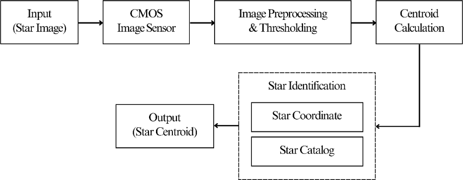
The algorithm starts by capturing the star images using prototype camera. The image preprocessing techniques are applied prior to the centroid calculation. Unlike conventional approaches that apply these techniques independently, the proposed method combines median filtering, thresholding method, and intensity-weighted centroiding in a coordinated manner to enhance robustness against noise while preserving star features. Then the obtained star coordinates are compared with the star catalogue to ensure that the stars captured are true.
The proposed method is evaluated through few tests using synthetic star images subjected to Gaussian and Salt-and-Pepper noise models to assess its accuracy and robustness under different conditions. In this study, Gaussian and Salt-and-Pepper noise are used as baseline models to represent continuous and impulse noise characteristics, respectively (Erkan & Kilicman 2016; Xu et al. 2020). These models enable controlled evaluation of centroiding performance under degraded SNR conditions, as an initial approximation of complex lunar surface imaging effects such as non-uniform illumination and regolith reflections. Additionally, the algorithm is constructed using conventional techniques, which are the median filtering, thresholding method and centroid calculation with the main contribution focusing on their combination and parameter selection to achieve improved robustness under degraded imaging conditions.
In this research, the point spread function (PSF) is used to simulate the optical blur introduced by a star camera system. Since real star images inherently contain some degree of blurring due to the optical and sensor characteristics of the camera, a Gaussian PSF is applied to synthetic star images to replicate this behavior. The Gaussian PSF approximates the way a point light source is spread out over several pixels on a detector. The Gaussian PSF model is defined as:
where σ is the SD of the Gaussian function, which controls the amount of blur. The Gaussian PSF or PSF kernel determines the area over which the function is applied. The Gaussian PSF is applied to the image, I(x,y), through convolution to simulate the blurred appearance of a star:
The kernel size of the Gaussian PSF should be sufficient to encompass the majority of the Gaussian’s energy (Chung 2007). For initial testing, a SD of σ = 1.5 is used with kernel size of 7 × 7. However, for a more realistic simulation, especially for star tracker applications where stars may appear larger and more diffused, higher values of σ = 2.0 to 2.5 can be used as well. These require larger kernels such as 11 × 11 or 13 × 13 to properly represent the PSF.
Fig. 2 illustrates the 2D Gaussian kernel as a bell-shaped surface is generated. The graph shows the smooth, symmetrical decay of intensity from the center outward, which is characteristic of the Gaussian function. This profile mimics how light from a distant star would spread when captured by a real optical system.
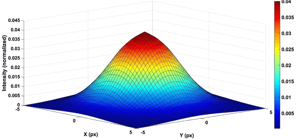
The shape of the bell curve is directly influenced by the value of the σ; a smaller σ results in a sharper and narrower peak, concentrating most of the intensity at the center, while a larger σ produces a broader and flatter peak, spreading the intensity over a wider area. In the case of a σ = 2.0 the kernel captures a wide enough region to realistically approximate the PSF of most moderate-resolution star trackers.
To enhance the quality of star images prior to centroid detection, a median filter model is applied to reduce background noise and isolate potential star regions (Hung et al. 2014). The median filter operates by sliding a window across the image and, at each position, replacing the central pixel with the median value of the pixel and its surrounding neighbors within the window (Patrice 2016).
As an example, consider 3 × 3 kernel:
The sorted values in this window are:
The median value is 38, which replaces the center pixel. The converted image becomes:
This process is repeated across the entire image, providing effective suppression of impulse noise and preserving edges, making it suitable for star field images with scattered bright blobs.
After denoising, the filtered image is binarized using global thresholding T to segment potential star regions from the background. The global threshold T is defined as:
α is a threshold factor, typically between 0 to 1, which determines the sensitivity of the segmentation and I is the intensity. A lower α allows more pixels to be classified as stars (foreground), while a higher α is more selective. A threshold factor was determined through trial-and-error testing within the range of 0.2 to 0.4. By evaluating detection performance, a value of 0.2 was selected as it provided the most accurate star blob segmentation with minimal noise.
Since the threshold is derived from the brightest intensity in the image, strong localized bright spots may influence the segmentation process and increase the possibility of false detections. However, under the simulated low-SNR conditions used in this study, the selected threshold factor was still able to distinguish most star regions from background noise with acceptable accuracy. The maximum intensity value, max(I), in the filtered image represents the brightest pixel, which is typically assumed to be part of a star. Multiplying it by α sets a dynamic threshold that scales with image brightness.
I(x,y) is the intensity of the pixel at position (x,y) in the filtered grayscale image. B(x,y) is the resulting binary image, where a value of 1 indicates potential star pixel (foreground) and a value of 0 indicates background. This method produces a binary image that highlights high-intensity regions that presumed to be star blobs while suppressing the lower-intensity background. The use of a dynamic threshold based on max(I) helps the algorithm adapt to different lighting conditions or brightness levels in the star images.
Although global thresholding is less adaptive compared to local (adaptive) thresholding, it is well-suited for this application because the image has already been filtered to reduce noise and background variation. The simplicity of global thresholding also makes it computationally efficient, which is advantageous in embedded or real-time systems such as satellite star trackers.
For each labelled star blob, the centroid is calculated to estimate its center. If for the case where all pixels have uniform mass, and the centroid is calculated as the geometric center of all pixels in the blob:
N is the number of foreground pixels in the blob and (xi,yi) are the coordinates of each pixel in the blob.
However, in real star images, the brightness of a star is not uniformly distributed, it typically forms a peak at the center and gradually decreases outward. To account for this brightness variation and achieve higher centroiding accuracy, the centroid can instead be calculated using an intensity-weighted approach also known as the Center-of-Mass method. This method utilizes the original grayscale (or denoised) image, where each pixel’s contribution to the centroid is proportional to its intensity, rather than treating all foreground pixels equally. The intensity-weighted centroid is given by:
I(x,y) is the pixel intensity (brightness) at location (x,y), and the summation is performed over all pixels in the labelled region.
To validate the accuracy of star detection and centroiding, the detected stars are cross-referenced with a known star catalogue. This process ensures that the identified stars correspond to real celestial objects, thereby enabling reliable attitude determination.
The validation process begins by referencing the existing star catalogue, which contains precise right ascension (RA) and declination (Dec) values for a wide range of stars. A subset of this catalogue is loaded into the system, providing known positions for comparison. To establish a geometric relationship between the detected star positions in the image and their actual coordinates, at least three reference stars are manually selected from the processed image. Their corresponding pixel coordinates are paired with known RA/Dec values obtained from the catalogue. This manual selection is performed to ensure that the detected star features correspond to actual stars rather than noise artifacts or other celestial objects, by directly validating them against catalogue data. However, this approach is not fully autonomous and is used here strictly for validation purposes. In practical star tracker systems, this step would be replaced by an automated star identification process.
An affine transformation is then computed using these reference pairs (House & Keyser 2020). This transformation accounts for translation, rotation, and scaling between the image and the celestial sphere, allowing the mapping of all detected centroids from pixel coordinates to sky coordinates. Eq. (7) represent the transformation using homogeneous coordinates:
is point in the homogeneous coordinates, M is the affine transformation matrix and ’ is the transformed point. After the transformation, the RA/Dec of all stars detected in the image are determined. These coordinates are then compared with the Hipparcos catalogue to identify and validate the stars (Perryman 2008). The nearest Hipparcos star number (HIP) in the catalogue is then assigned as the matching star for each detected object. This approach provides a one-to-one mapping and enables verification of detection accuracy. By matching observed star centroids with known catalogue entries, this method not only confirms the identity of stars in the image but also facilitates attitude determination, as the known positions of matched stars can be used to compute the orientation of the imaging platform.
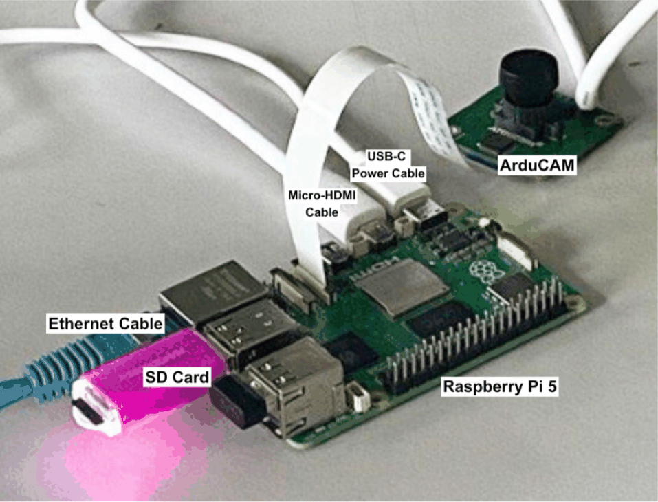
To ensure accurate image acquisition for star detection and centroiding, selecting an appropriate camera module is crucial. For this study, the ArduCAM 2 MP OV2311 global shutter monochrome camera module (Arducam, Nanjing, China), a MIPI CSI-2 compatible camera designed for Raspberry Pi platforms is chosen. The assembly of the star camera is shown in Fig. 3 and the camera specifications shown in Table 1.
To simulate an orbital environment, a custom-made aluminum profile jig was constructed to provide a rigid, light-shielded framework for the hardware. Within this setup, the camera is positioned facing a monitor, which serves as the primary visual source by displaying the Stellarium star field images, shown in Fig. 4. This setup allows the system to capture realistic star patterns while maintaining full control of the ground-testing environment.
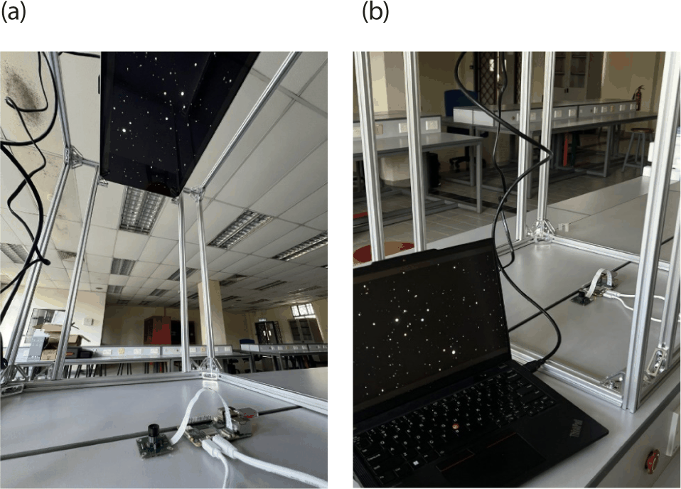
This method allowed for controlled testing but does not fully reflect the atmospheric effects, light pollution, and the sensor’s response to faint stars. Capturing images from the screen alone may not fully reflect real-world challenges. To address this, the images were further modified by introducing noise models which are: Gaussian noise and Salt-and-Pepper noise. Once captured, the raw or processed images were transferred and logged for subsequent preprocessing and centroiding algorithm evaluation.
3. RESULTS
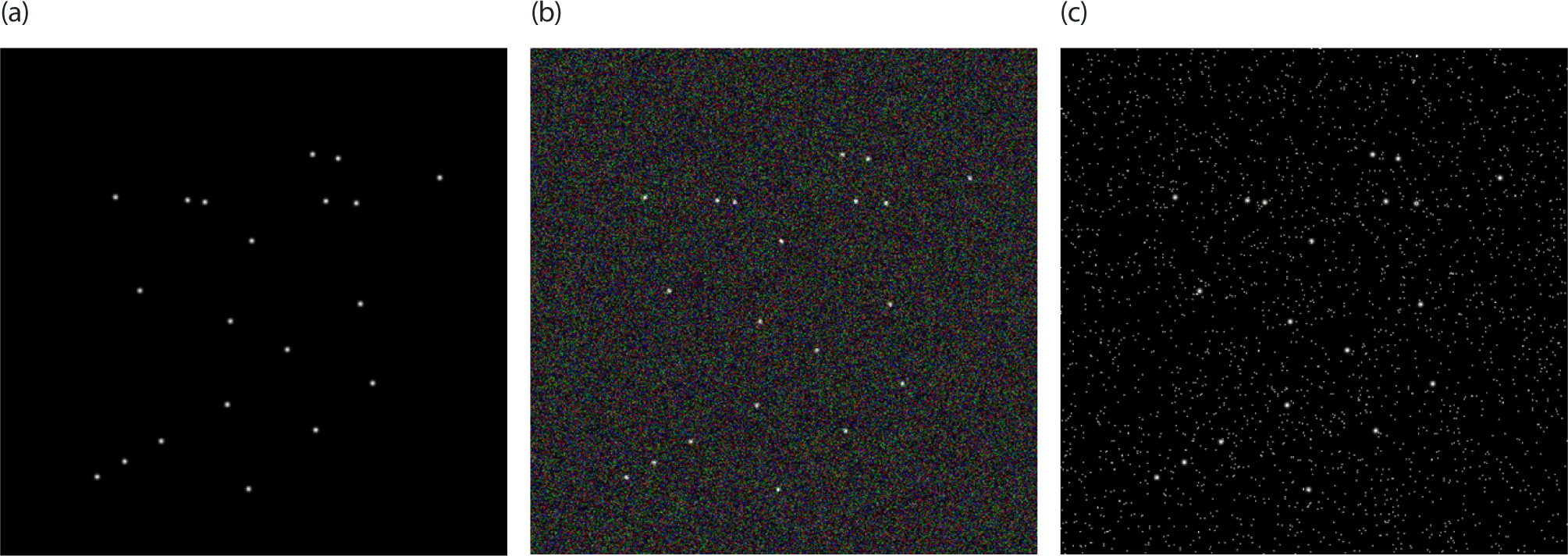
In this section, the proposed star detection and centroiding algorithm is evaluated using synthetic star images. Each test image contains random 20 simulated star blobs, and two different noise models are applied to assess the robustness of the algorithm under varying conditions. The objective is to analyze the accuracy of centroid detection by comparing the detected positions against ground truth values and benchmark the performance against existing methods. The two noise models implemented are Gaussian noise model to simulate the random fluctuations typically observed in space-based imaging systems, and Salt-and-Pepper noise model to introduce sparse but high-contrast noise, representing faulty pixel behavior or cosmic ray impacts. For ground truth, the synthetic star blobs image is generated in Fig. 5(a)–5(c) shows the image under Gaussian noise and Salt-and-Pepper noise, respectively.
To evaluate the centroiding accuracy of the proposed algorithm, the Euclidean distance, or position error, between the detected coordinates and ground truth was computed for all 20 stars under Gaussian noise conditions. Moreover, we also plotted the detected star coordinates of proposed algorithm against the ground truth for a clearer comparison. The coordinate data comparison is illustrated in Fig. 6(a) and 6(b).
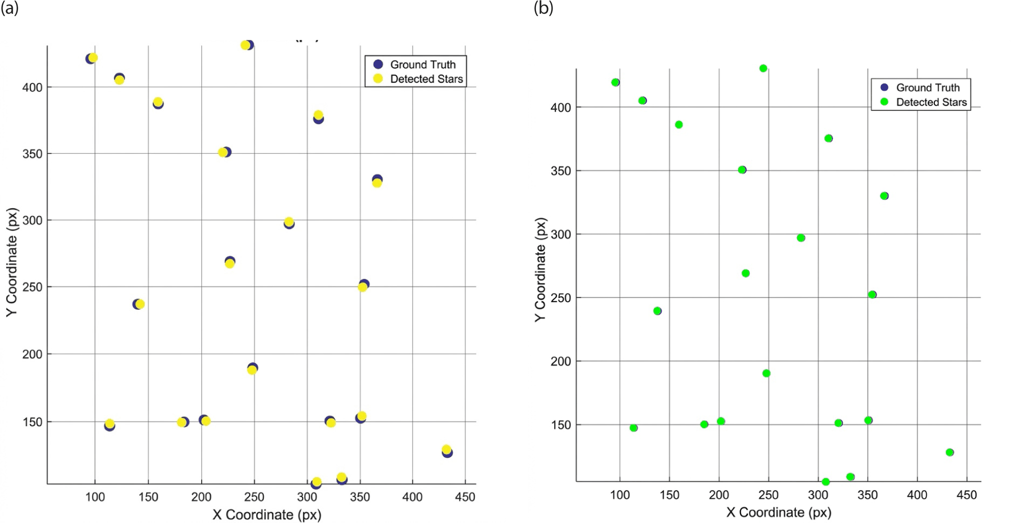
The results show a strong match between the detected star positions and the ground truth. In most cases, the difference is only around 1 to 3 pixels, which suggests that the centroiding method achieves near sub-pixel accuracy.
After preparing the synthetic star images, we conducted tests using the proposed algorithm and compared its performance with two existing techniques: the SSA and the COM method. Fig. 7(a) illustrates the centroiding results under Gaussian noise conditions, while Fig. 7(b) presents the results under Salt-and-Pepper noise.
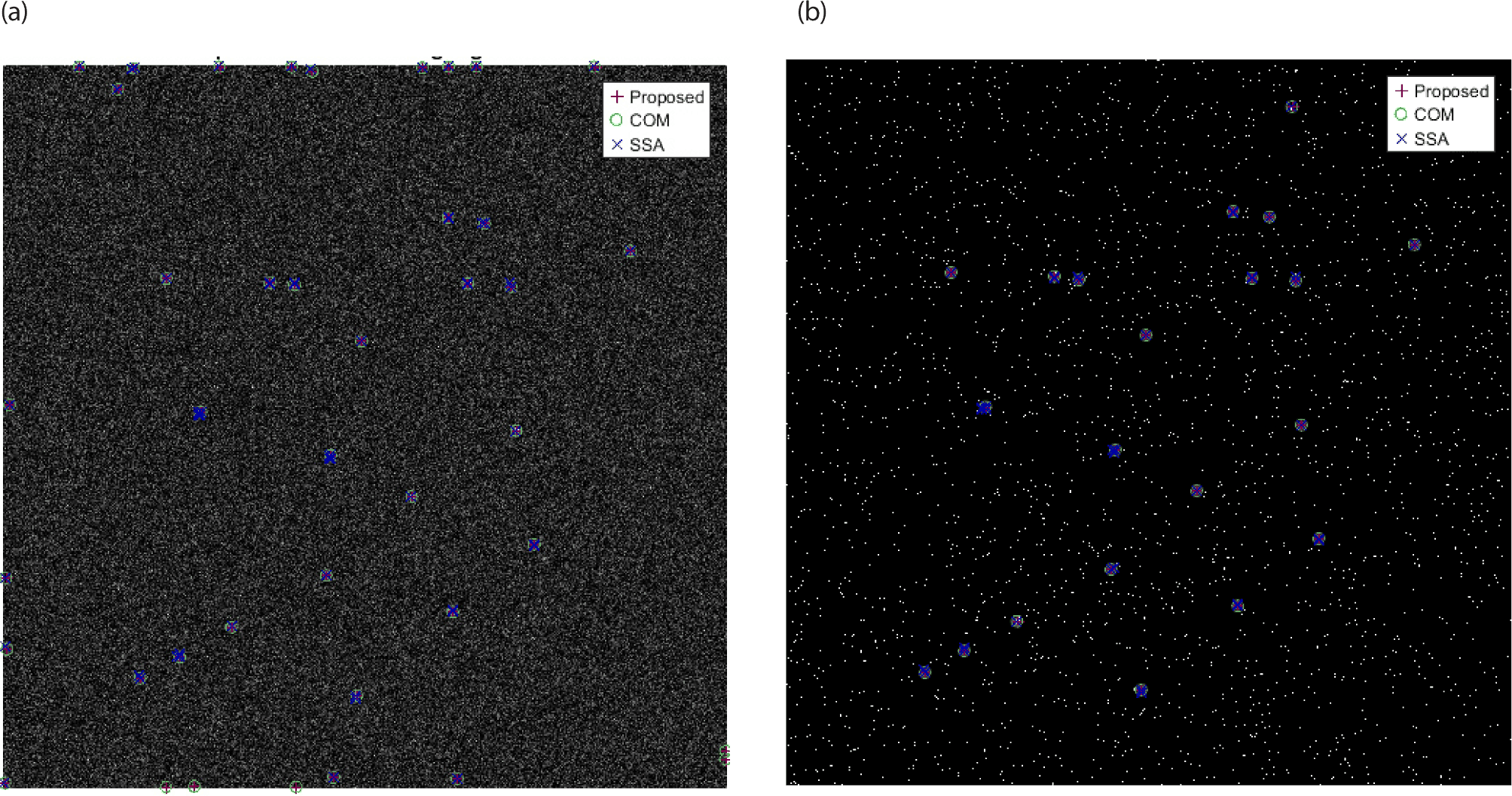
The overlay visualization illustrates the spatial distribution of detected centroids on top of the grayscale image of the star field. In the figures:
-
Red plus signs denote the detected centroids using the proposed method,
-
Blue crosses represent detections from the SSA method, and
-
Green circles correspond to the SSA method.
The result, shown in Fig. 8, compares the per-star error distance for the COM, SSA, and the proposed method. From the chart, it is evident that the proposed method consistently maintains low error distances, mostly within 1 to 1.5 pixels, across all stars. In contrast, COM shows the highest variance and largest error distances, frequently exceeding 3 pixels and reaching up to 3.60 pixels. Proposed method achieves better consistency than SSA but still fluctuates, with distances typically ranging between 1 and 2.5 pixels.
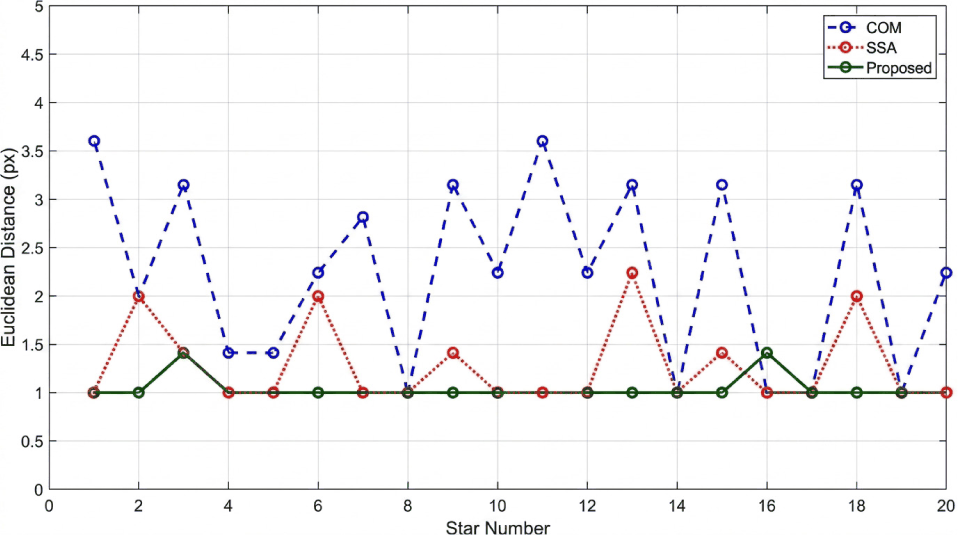
Proposed method outperforms both, achieving the lowest distance on nearly all the star positions. While these methods still detect the majority of stars, the centroids from the COM and SSA approaches show slightly larger positional differences. This can be seen in the line graph, where both methods generally have higher average Euclidean distance values. The accuracy analysis for the three methods was recorded in Table 2.
| Metrics (average) | COM | SSA | Proposed method |
|---|---|---|---|
| MSE | 7.20 | 1.80 | 1.20 |
| RMSE | 2.68 | 1.34 | 1.09 |
| Euclidean distance | 2.63 | 1.28 | 1.08 |
Based on the comparison table, the proposed method clearly performs better than both the COM and SSA in terms of accuracy. The average MSE dropped from 7.20 with COM to 1.80 using SSA and further improved to 1.20 with the proposed method. A similar trend can be seen in the RMSE and Euclidean distance values, where the proposed method consistently records the lowest error. Specifically, the Euclidean distance is reduced from 2.63 (COM) to 1.28 (SSA), and down to just 1.08. These results suggest that the proposed method offers more precise and reliable centroid detection compared to the other two methods tested.
To evaluate the efficiency of each algorithm, we plotted the runtime under both noise models in a bar chart, shown in Fig. 9. The chart provides a visual comparison of the computational cost for COM, SSA, and the proposed method.
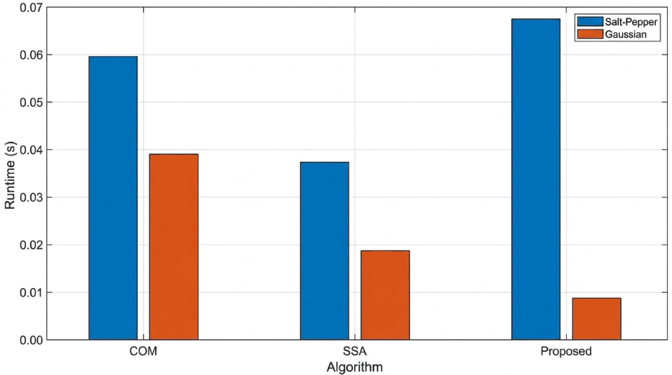
In Salt-and-Pepper noise environment, SSA has the fastest runtime of 37.5 milliseconds, followed by COM at 59.6 milliseconds. The proposed method took 67.7 milliseconds, slower than SSA. This increase in time is mainly due to the additional image preprocessing steps performed prior to star detection. However, the processing time of 67.7 milliseconds per frame remains within practical limits for real-time star sensor systems. Typical onboard star trackers operate at update rates between 1 and 10 Hz, corresponding to 100–1,000 milliseconds per frame (Qiao et al. 2012). Meanwhile in Gaussian noise environment, the proposed method outperformed both benchmarks with the lowest runtime of 8.7 milliseconds, showing superior computational efficiency. SSA followed with 18.8 milliseconds, while COM had the highest runtime at 39.1 milliseconds. The bar chart clearly shows that the proposed method is consistently efficient, especially under Gaussian noise, where it is over 4 times faster than COM and more than 2 times faster than SSA.
Although the proposed method shows higher runtime than SSA under Salt-and-Pepper noise, it consistently achieves better accuracy and lower false detection rates across both noise conditions. This indicates that the method provides a more reliable centroiding performance while maintaining acceptable computational efficiency. Therefore, the proposed approach offers a better overall trade-off between accuracy, robustness, and runtime compared to the other methods.
For initial testing using real star images, we captured the image using the star camera prototype and obtained its star data: the RA and Dec coordinates and HIP. These data are important in this experiment because we will use at least three stars’ data as the reference, as shown in Table 3.
| Star # | Pixel coordinate (x,y) | RA-coordinate (°) | Dec-coordinate (°) | HIP |
|---|---|---|---|---|
| 20 | 328.81, 437.46 | 185.0822 | 26.61975 | 60170 |
| 30 | 364.46, 394.72 | 186.0772 | 26.09861 | 60514 |
| 40 | 416.7, 383.71 | 187.159 | 26.22697 | 60880 |
The noise model, Gaussian noise and Salt-and-Pepper noise, is also included in this experiment. The star image can be seen in Fig. 10(a).
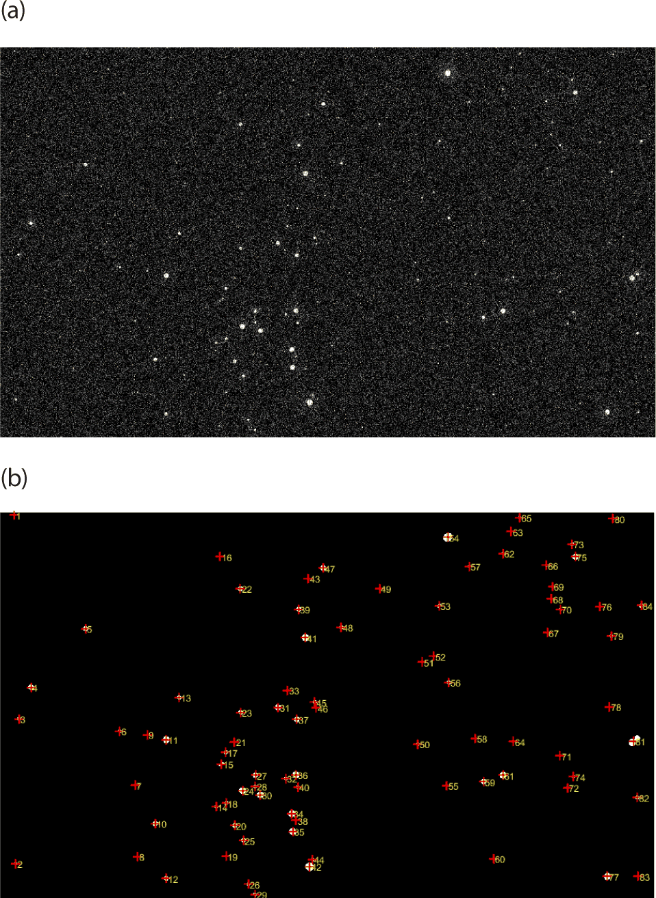
By using the proposed method, the noise in the background was successfully removed and the centroid coordinates were calculated. As shown in Fig. 10(b), the center of each star is marked by a red marker and each star is labeled with numbers. The detected stars were then compared with the Hipparcos catalogue to match the stars. This testing is to ensure that the algorithm can actually detect real stars and their coordinates. Some of the detected stars and its angular distance error are recorded in Table 3, full data is available in Appendix.
Overall, the algorithm successfully matched 53 blobs with the star catalogue using three reference stars. The angular distance error shown in Table 4 represents the difference in RA/Dec coordinates between the detected stars and those in the catalogue. Based on the results, we observe that when the error is below 0.1°, the algorithm can still correctly match detected stars with their corresponding HIP entries. This suggests that the proposed method is capable of detecting real stars accurately.
4. CONCLUSION
This study presented an enhanced centroiding algorithm for star detection and attitude determination, specifically optimized for lunar mission environments. The proposed method offers reliable star detection with strong resilience to noise and efficient processing time, making it well-suited for potential use in onboard star sensor systems. To ensure this method is improved and reliable than other methods, we took the test with other two benchmarks: COM and SSA method. The testing was done using synthetic star images under two different noise conditions: Salt-and-Pepper and Gaussian. Across both cases, the proposed method produced the lowest position error or average Euclidean distance values than the other two methods, indicating star centroid with higher precision. To further evaluate the proposed method’s real-world capability, a test using a real star image captured through the star camera was conducted. The angular distance error of matched stars remained below 0.1°, confirming the method’s practical accuracy in identifying real stars.
To further improve the algorithm’s applicability for real space missions, several future directions are proposed. Firstly, incorporating additional noise models, such as solar radiation and surface reflection noise, would enhance the algorithm’s resilience under harsh lunar conditions. To remove those noise models, the adaptive thresholding will be considered as part of the future works to obtain a better and more stable segmentation results under varying illumination conditions. Additionally, integrating real star catalogues with more real star images will further ensure the algorithm’s reliability and alignment with actual celestial references. For real mission applicability, adaptations could be made for spaceflight and lunar navigation systems, such as integrating pattern recognition algorithms, enabling fully autonomous Lost-in-Space operation without manual selection of reference stars. Through these advancements, the proposed algorithm holds promise as a dependable component in onboard star sensors for autonomous navigation in lunar exploration missions.


