
 PDF Download
 PubReader
 Export Citation
 Email the Author
 Share Facebook
 Share Twitter
 Cited by 0 Article
 Metrics (View:1,973)










1. INTRODUCTION
Initial Orbit Determination (IOD) is a crucial step in the fields of space object surveillance and space situational awareness. It aims to rapidly and accurately estimate the initial orbital parameters of a space object using limited observational data. The accuracy and reliability of its results directly impact the effectiveness of subsequent tasks such as orbit refinement, object correlation, and collision warning (Kazemi et al. 2024).
With the rapid development of activities in near-Earth orbit and deep space exploration, the number of space objects has grown dramatically. As of October 21, 2025, the number of space debris pieces sized between 1 cm and 10 cm is estimated at 1.2 million, while only 43,510 objects are tracked by the space surveillance network (ESA 2025). Optical angle-only observation has become a primary means for space object surveillance due to its significant advantages: the ability to track multiple objects simultaneously, high angular measurement accuracy, relatively low equipment cost, and high observation efficiency. Compared to ground-based observation, space-based optical observation platforms (deployed on spacecraft such as satellites) offer unique benefits: they are free from atmospheric disturbance and day-night cycle limitations, enabling near-global, all-weather coverage; and they can observe high-altitude objects (e.g., GEO) at close range, significantly improving observation accuracy (Qiao et al. 2006; Yu et al. 2006; Li et al. 2018; Zhao et al. 2022).
Angle-only IOD has been studied for over two centuries. As classical IOD methods, the Laplace algorithm and the Gauss algorithm both aim to obtain orbital parameters by solving an eighth-order polynomial equation concerning the geocentric distance of the object at the central observation epoch (Vallado & McClain 2013). Although the goal is the same, they differ in the theoretical basis for constructing this equation and the technical approaches to eliminating unknown variables within it. Advancements in computer technology have significantly enhanced iterative computation efficiency, promoting the development of a new generation of IOD algorithms. Among them, Gooding, based on the unified form of the Lambert equation proposed by Lancaster, constructed an IOD method that minimizes the direction vector residuals (Gooding 1990). Similarly, Sang et al. also utilized the Lambert equation to propose a range-search algorithm that integrates multi-directional observation data (Sang et al. 2017). However, the Lambert equation method inherently requires a certain observation arc length. When dealing with Very Short Arc (VSA) data, where the observation arc is less than 1% of the orbital period, the numerical stability and orbit determination accuracy of such methods significantly degrade (Zhang et al. 2024). In recent years, artificial intelligence (AI) methods have also been explored for IOD. Lee et al. applied machine learning to IOD of unknown satellites, though requiring additional range information (Lee et al. 2018). Agostinelli et al. combined metaheuristics with AI to achieve IOD from VSAs (Agostinelli et al. 2024). Despite these efforts, AI-based approaches face inherent limitations such as lack of interpretability, strong dependence on training data, and difficulty in quantifying uncertainty, which are critical concerns in safety-critical space applications (Kazemi et al. 2024).
The admissible region (AR) algorithm, based on energy and angular momentum constraints, defines the feasible solution space for Earth-bound orbits in the range–rate space, forming the core foundation of IOD. Early research defined the physical boundaries of the AR through the two-body problem (Milani et al. 2004). DeMars & Jah innovatively probabilized it into a Gaussian Mixture Model (GMM), significantly improving the processing accuracy for short-arc data through probability density iterative optimization (DeMars & Jah 2013). The AR algorithm has demonstrated strong adaptability in multiple scenarios: in space debris monitoring, the Constrained Admissible Region (CAR) incorporates orbital parameter constraints, effectively enhancing solution robustness under optical/space-based observation in noisy environments (Tommei et al. 2007; Fujimoto & Scheeres 2013; Guo et al. 2024); in short-arc data association, Fujimoto et al. proposed an optical observation short-arc association method based on AR probability distribution overlap judgment, achieving initial association and orbit determination without iteration by mapping each arcs AR to the Poincaré orbital space and computing their intersection (Fujimoto & Scheeres 2012). With its synergistic mechanism of physical constraints and probabilistic modeling, AR has become a key technology for space object orbit determination.
With its synergistic mechanism of physical constraints and probabilistic modeling, the AR has become a key technology for space object orbit determination. Statistical data show that near-circular orbits with eccentricities below 0.05 constitute up to 96.3% of all space objects, forming the main body of space object types (Space-Track.org 2025). However, when space-based optical observation is applied to the IOD of such objects, the AR algorithm exhibits a specific limitation. Under the circular orbit assumption, certain relative geometric configurations between the space-based platform and the target—such as coplanar orbits with aligned or opposite velocity directions—cause the constraint equations to yield multiple mathematically valid solutions. Only one of these corresponds to the true orbit, while the others are erroneous solutions that satisfy all physical constraints but are geometrically induced. This inherent multi-solution problem has not been systematically addressed in prior AR-related research and hinders the practical application of the algorithm in space-based surveillance systems.
To address this gap, the present study analyzes the generation mechanism of these erroneous solutions and proposes a novel Relative Variance-based Single-Parameter Solution Screening (RV-SPSS) method. The key novelty of this approach lies in constructing solution sets from multiple observation point pairs with varying geometric characteristics. By leveraging the principle that the true solution is invariant under geometric variations, while erroneous solutions are highly sensitive to such changes, the method uses the relative variance of the solution set as a statistical criterion to identify and eliminate erroneous solutions. This introduces a geometry-diversity-based screening strategy that enhances the reliability of initial orbit determination in complex space-based observation geometries.
The proposed method significantly increases the probability of avoiding erroneous solutions, thereby reducing the likelihood of large errors in the orbit determination results. Finally, the algorithms performance—including success rate and solution accuracy—is validated using space-based simulation data across Low Earth Orbit (LEO), Medium Earth Orbit (MEO), and Geostationary Earth Orbit (GEO) scenarios.
2. DATA AND METHOD
The core data acquired by a space-based optical observation platform consist of the observation epoch ti, the objects right ascension αi and declination δi in the platforms observation coordinate system, and the instantaneous position vector Ri and velocity vector Ṙi of the observer in the geocentric celestial inertial frame, which are determined via onboard GNSS and precise orbit determination systems. From the right ascension and declination measurements, the line-of-sight unit vector λi from the observer to the object can be constructed. Its Cartesian components in the geocentric inertial frame are expressed as:
This unit vector defines the line-of-sight direction from the observer to the object at epoch ti.
The core of IOD is to solve for the initial orbital state of the object. The unknowns are the objects position vector ri and velocity vector ṙi (or the equivalent Keplerian elements) at the observation epoch. Based on geometric relations, the object position satisfies the following equation involving the observer position, line-of-sight direction, and the unknown slant range ρi:
The motion of both the object and the observer follows the two-body dynamical model, with their accelerations governed by the central body (Earth) gravitational attraction:
Where μ is Earths gravitational constant. The object velocity vector can be obtained by differentiating the geometric relation:
In recent years, methods for initial orbit determination using angle and angle-rate measurements of space objects have been developed. Advancements in CCD technology allow telescopes to acquire angle measurements at frequencies of 10 Hz or higher with improved accuracy, enabling precise estimation of angle rates (Bloch & Rast 2007). Theoretically, based on single-epoch angle and angle-rate measurements, the objects position and velocity states can be expressed as functions of range and range rate.
Building on this, Milani et al. introduced the concept of the AR for space objects. For near-Earth object surveillance, under the two-body motion assumption, limited angle data can determine the feasible solution interval—the AR—for the parameters of a object. If further constraints (such as limits on orbital semi-major axis and eccentricity) are applied, a more restricted CAR can be obtained. There is no strict boundary between AR and CAR; typically, CAR refers to the solution set when a larger number of constraints are used. The core idea is to utilize the observation information (right ascension α0, declination δ0, and their rates , ) at a specific Time of Interest (TOI), combined with the orbital characteristics of the space object, to confine the directly unobservable range ρ and range rate to a two-dimensional feasible solution region—the AR. This region is constructed through the following key constraints: orbital energy constraint, semi-major axis constraint, and eccentricity constraint.
The orbital energy ε of an Earth-orbiting object must satisfy the two-body motion condition. From the geocentric inertial position vector r and the velocity vector ṙ, and using the topocentric spherical coordinate representation, the energy equation is derived:
After simplification, an explicit relationship involving ρ and is obtained (DeMars et al. 2012):
Where w1 is the projection coefficient of the observer velocity onto the line-of-sight direction, and F(ρ) is a function of ρ (Zhao 2020). Given the energy ε, one can solve for:
Using the elliptical orbit constraint, solution curve boundaries and their interior region D1: ε < 0 can be generated.
Using the relation between semi-major axis a and energy, ε = –μ / (2a), combined with the energy equation:
Substituting into the energy constraint equation yields the solution boundary curve corresponding to the semi-major axis upper limit, with its interior region satisfying D2: a ≤ amax.
From the angular momentum h = r × ṙ and the eccentricity formula:
A fourth-order polynomial equation in ρ and is derived:
The coefficients ai are functions of ρ. Given an eccentricity upper limit emax, solving this equation yields the boundary, with its interior satisfying D3: e ≤ emax.
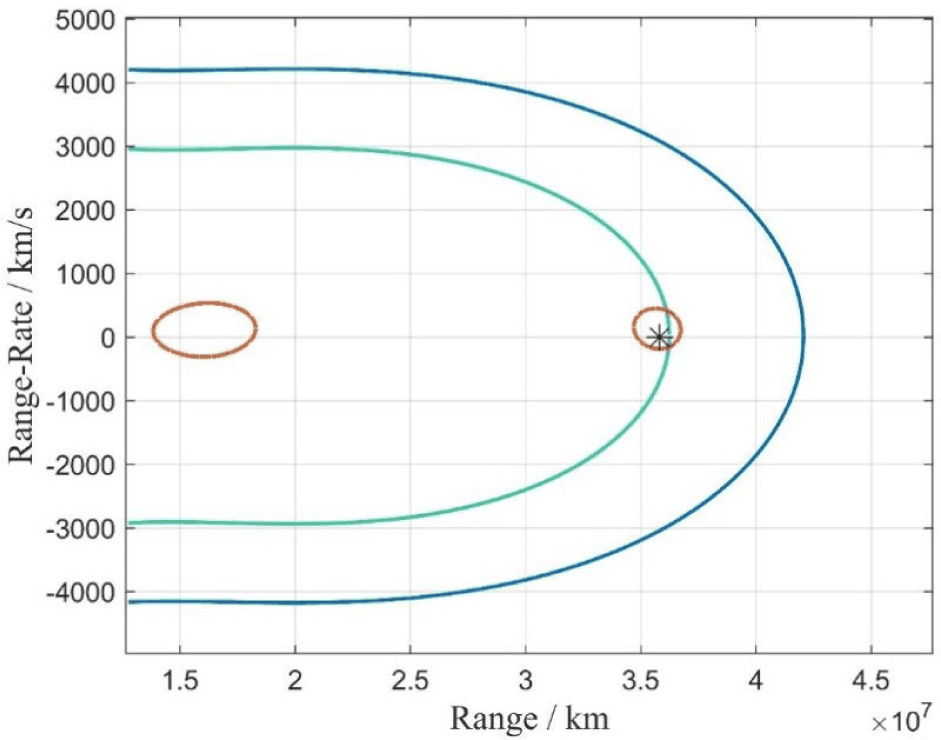
The intersection of the above constraint regions, D1 ∩ D2 ∩ D3 (i.e., the energy, semi-major axis, and eccentricity constraint regions), forms a compact two-dimensional solution domain. As shown in Fig. 1, the blue curve represents D1; the green curve represents D2; the red curve represents D3; and the asterisk marks the objects true solution. This domain contains the objects true orbital parameters (ρ, ), providing a prior solution space for subsequent probabilistic modeling (e.g., uniform distribution assumption) or filtering estimation. It can be seen from Fig. 1 that the feasible region corresponding to the eccentricity constraint is divided into two areas: one contains the true solution, while the other constitutes an erroneous solution that needs to be eliminated in automated processing.
Utilizing sparse observation data for Initial Orbit Determination alleviates constraints on observation equipment and conditions but inevitably increases solution uncertainty. The multi-solution dilemma inherent in space-based angle-only IOD serves as clear evidence—computed orbits, although not the true object trajectory, can precisely fit the observational geometric configuration and the dynamical relationships implied by the condition equations, rendering erroneous solutions and the true solution indistinguishable and ultimately amplifying orbital parameter errors. This dilemma directly stems from the lack of range measurement information in angle-only observations.
For space-based observation of near-circular orbit objects, the AR algorithm can produce erroneous solutions, which severely impacts the subsequent determination of orbital parameters. The cause for the appearance of these erroneous solutions is briefly explained below. For a circular orbit (eccentricity zero), the eccentricity constraint simplifies significantly. Eq. (9) can be reduced to:
Combining with the semi-major axis and energy relationship, it further simplifies to:
Furthermore, due to the circular orbit, h = a2ω, where ω is the mean angular velocity, yielding:
Eq. (13) establishes the relationship between semi-major axis and mean motion under the circular orbit assumption. This forms the basis for the single-parameter initial orbit determination method discussed in the following section.
First, assume an initial semi-major axis â. The theoretical mean motion n can be obtained via Keplers law:
Next, the computed value of mean motion n2 is given by â and ri:
From Eqs. (4) and (5), the objective function can be constructed as:
when f(â) = 0, the function converges, and the resulting â is the solution. In the above equation, ri is unknown and needs to be obtained using ρi. Utilizing the geometric relationship between the telescope and the object, ρi can be expressed in terms of â and other known quantities:
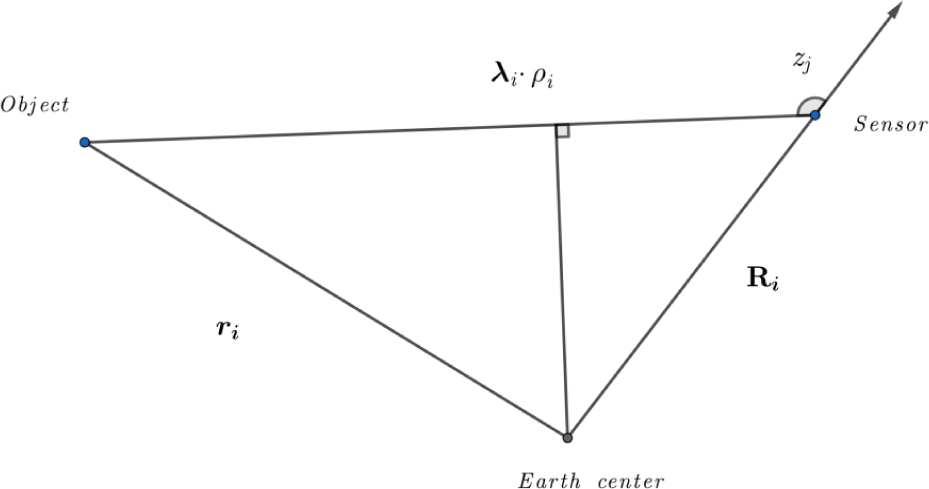
where z is the zenith distance, whose geometric relationship is illustrated in Fig. 2.
Although Eq. (13) suggests a one-to-one correspondence between a and ω under ideal conditions, the practical solution of Eq. (16) can yield multiple roots. This occurs because is strictly decreasing in â, while n2(â) is generally non-monotonic. The non-monotonicity of n2(â) arises from the dependence of r1 and rend on â via the slant range ρ (Eqs. (17)–(19)), and the fact that the dot product r1 · rend involves the cosine of the angle between two geocentric position vectors. As â varies, this angle can change non-linearly, causing n2(â) to increase or decrease in a complex manner. Consequently, the decreasing curve of n1(â) may intersect the non-monotonic curve of n2(â) at two distinct points, yielding two different â values that satisfy f(â) = 0. One corresponds to the true orbit; the other is a mathematically valid but physically incorrect spurious solution—referred to as an erroneous solution.
In essence, the apparent angular rate derived from angle-only measurements depends not only on â but also on the instantaneous line-of-sight geometry. Different combinations of â and geometry can produce the same observed angular rate, leading to multiple mathematical solutions that satisfy all physical constraints. This is the core reason for the multi-solution problem.
In the space-based scenario, the platform itself moves along a Keplerian orbit, introducing additional geometric variations that make the dependence of n2(â) on â more intricate. This increases the chance of multiple intersections, as illustrated by the examples in Section 2.3.3.
Existing space-based long-range surveillance platforms primarily operate in near-circular orbits, and small-eccentricity orbits offer excellent performance in terms of the number of observed objects and observation arc length for low-Earth orbit multi-object surveillance (Zhao 2020). The space-based observation discussed in this paper is also based on long-range near-circular orbit observation platforms. The key difference between space-based and ground-based observation lies in the different motion laws followed by the observation platform itself. The ground-based platform is subject to Earth’s rotation, whereas the space-based platform, like the observed object, follows Keplers laws. This distinction makes the single-parameter algorithm more prone to generating erroneous solutions due to geometric configurations when applied to space-based observation data.
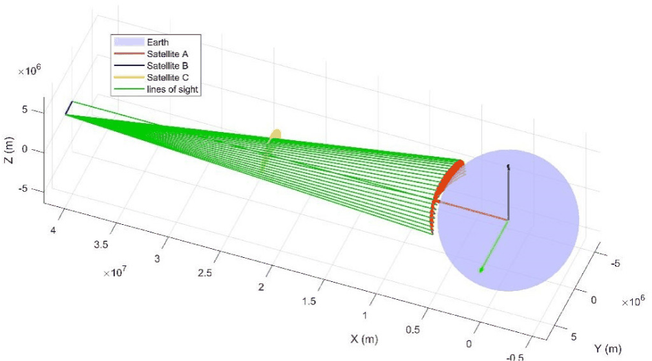
For the objective function Eq. (17), when the semi-major axis value equals the observation platforms own aobs, the function also equals zero. This solution is considered a trivial solution and can be filtered out by applying a slant range threshold. However, beyond this, consider the following geometric configuration: the object orbit and the observation platform orbit are coplanar, with velocity directions aligned. In this case, within the reasonable range of the independent variable, both and n are monotonically decreasing functions, and two solutions exist that satisfy the objective function equaling zero (the true solution and the trivial solution). If the orbital elements of the two satellites remain unchanged, but their velocity directions are opposite, within the same value range, remains unchanged, but n exhibits a minimum point, and the extremum is zero. The geometric configuration of the observation line of sight changes continuously, and the corresponding objective function also changes. To intuitively understand this characteristic, Fig. 3 shows a hypothetical space-based observation scenario, and Fig. 4 shows the corresponding function variation.
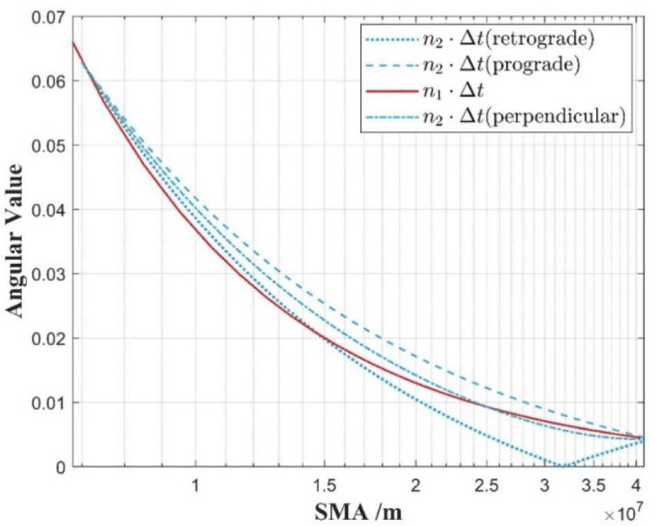
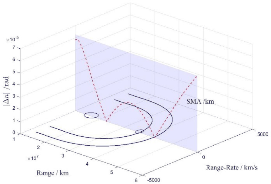
As can be seen from Fig. 4, during the process of the observation platforms orbital plane changing from 0° to 180°, geometric configurations exist that cause the objective function to produce erroneous solutions. These solutions conform to physical laws and are difficult to distinguish from the true solution. Fig. 5 demonstrates the corresponding effect of combining the AR and the single-parameter algorithm. The x-axis in the figure is a shared coordinate axis. It can be observed that both algorithms yield two solutions, one true and one erroneous. However, the solutions from the two algorithms are not entirely consistent. This discrepancy arises because the meanings of the solutions differ: one represents the slant range in the AR algorithm, and the other represents the semi-major axis in the single-parameter algorithm. The figure shows that erroneous solutions corresponding to the single-parameter algorithm exist within the AR. Such erroneous solutions are not limited to the example geometric configuration. Therefore, a method to eliminate erroneous solutions is needed to enable the AR algorithm to be better applied to space-based angle-only initial orbit determination.
Due to its concise and intuitive form, the single-parameter algorithm was chosen as the basis for improvement in this paper to screen between erroneous and true solutions. Through the above analysis, it can be found that the value of erroneous solutions is influenced by the observation geometric configuration. This key point forms the core of the algorithm improvement proposed in this paper. Additionally, the J2 term is introduced as a perturbation correction term to improve the accuracy of angular velocity calculation. Finally, to reduce the impact of observation errors on the results, a noise reduction data preprocessing method is introduced.
In the initial orbit determination process, to effectively identify and eliminate erroneous solutions, this paper constructs multiple sets of observation data with varying geometric configurations by changing the observation arc length, start/end times, or a combination of both. Based on the key characteristic that the true solution is consistent across different observation geometries, whereas erroneous solutions are sensitive to such geometric changes, to effectively distinguish between them, geometric configurations with significant differences need to be constructed to amplify the distinction in solution set responses. To this end, this paper systematically selected six observation combinations aimed at maximizing geometric diversity. The selection primarily considered two key dimensions: arc length (shortest, medium, longest) and the relative position of the combinations central time within the observation time window (earliest, middle, latest). Consequently, the following six pairs were chosen:
Based on the method in Section 2.3.2, the orbital semi-major axis can be estimated using any two observation points. Therefore, six different data combinations can be extracted from one observation arc segment, solved separately to form a set of semi-major axis solutions {a1,1, a2,1, ..., a6,1}. If multiple solution groups exist, all solution sets can be represented as{a1,1, a2,1, ..., a6,1}, ..., {a1,m, a2,m, ..., a6,m}. It should be noted that when the number of data points is insufficient to select point pairs according to the above scheme, all possible combination pairs can be used as the selection scheme.
The true solution typically does not fluctuate significantly with changes in geometric configuration, whereas erroneous solutions are sensitive to changes in observation conditions. To characterize this difference, the variance within each solution set can be calculated to evaluate its dispersion (relative variance, as shown in Eq. (20), is used to avoid the influence of the expected value, where s̅ represents the mean of the solution set). Solution sets with smaller variance have higher stability and are more likely to correspond to the true orbit; solution sets with larger variance are judged as erroneous and excluded.
Furthermore, the existence of trivial solutions cannot be ignored. Especially when the zenith angle is less than 90°, their numerical values are less affected by geometric configuration, making it difficult to effectively eliminate them using the aforementioned variance analysis. Therefore, this paper incorporates a slant range ρ judgment threshold: if the solved slant range is below a positive number close to zero, it is considered a trivial solution, and that solution set is directly excluded.
To validate the rationality of the proposed six-group observation point selection scheme, the following comparative experiment was designed. The experiment aimed to systematically compare this scheme with two control schemes—the “scheme using only two points near the start and end times” (2-group scheme) and the “scheme using all possible point pairs” (full combination scheme)—in terms of performance when generating single-parameter solution sets.
The experiment utilized simulation data from three representative orbit types (LEO, MEO, GEO), with example orbital parameters shown in Table 1. For each orbit type, 100 repeated experiments were conducted. In each repeated experiment, an independent set of Gaussian random noise with a mean of 0 and a standard deviation of 3 arcseconds was generated and added to the simulated angle observation sequence to simulate the randomness of actual observation errors. Subsequently, for the same noise-added observation arc segment, the above three point-pair selection strategies were applied in sequence to solve the orbital semi-major axis based on the single-parameter method, forming the corresponding solution set S. The relative variance RV (measuring stability), mean, and average single computation time for each strategys solution set were recorded.
The experimental results are shown in Table 2. In terms of solution stability, for all orbit types, the relative variance of the solution sets from the 6-group scheme was significantly lower than that of the 2-group scheme, indicating smaller dispersion and stronger stability. Simultaneously, its stability was comparable to that of the full combination scheme. In terms of computational efficiency, the time consumption of the 6-group scheme, although slightly higher than the 2-group scheme, was far lower than the full combination scheme. For example, in the LEO scenario, the six-group scheme took 0.29 seconds, while the full combination scheme took 56.40 seconds, representing an improvement in computational efficiency of over two orders of magnitude.
Overall, the six-group scheme achieves an optimal balance between stability and efficiency, significantly improving solution set stability (compared to the 2-group scheme) while its computational cost is far lower than the full combination scheme. Therefore, adopting this scheme as the core strategy for constructing multi-geometry-configuration solution sets is reasonable and efficient.
Random noise in optical observation data is a key factor affecting the accuracy and solution set stability of initial orbit determination algorithms. To suppress noise, eliminate gross errors, and provide a smooth and reliable observation sequence for subsequent calculations, this paper employs a cubic polynomial fitting method to smooth the right ascension and declination observation sequences separately. Given the short observation arc, the objects celestial coordinates change smoothly. Using the time offset relative to the first observation epoch as the independent variable, the following fitting model is constructed:
The polynomial coefficients are obtained through least squares estimation, and then the smoothed values , at each epoch are calculated. To eliminate the influence of gross errors, an iterative processing strategy is adopted: after calculating the residuals at each observation point, outliers are identified and eliminated based on the Pauta criterion (3σ criterion). Polynomial fitting is then repeated using the remaining points, iterating until no gross errors remain, ultimately obtaining a clean, smooth observation sequence.
To systematically evaluate the effectiveness of this preprocessing method, a controlled experiment was designed. The experiment used the same sensor and object orbital parameters (LEO, MEO, GEO) as in Section 2.4.1. Under noise levels of 0, 0.5, 1, 2, 3, 4, 5, 6, 7, 8 arcseconds, the following three processing methods were compared: 1) No noise reduction (N); 2) The polynomial fitting method of this paper polynomial fitting (PF); 3) Iterative Reweighted Least Squares (IRLS). Each experimental group underwent 100 Monte Carlo repetitions, using the relative variance (RV) of the solution set as the evaluation metric, and distinguishing between correct solutions (small RV and orbital parameter error < 200 km) and erroneous solutions.
The experimental results are shown in Figs. 6–8 (corresponding to LEO, MEO, GEO, respectively). The horizontal axis represents noise level, and the vertical axis represents relative variance (exponential coordinates for 0–1 arcsecond, linear coordinates for 1–8 arcseconds). Blue, green, and red lines represent no noise reduction, polynomial fitting, and IRLS methods, respectively. Circular markers indicate erroneous solutions, square markers indicate correct solutions, and star markers indicate conditions under which the relative variance of the correct solution is smaller than that of the erroneous solution, meaning the algorithm can effectively eliminate erroneous solutions.
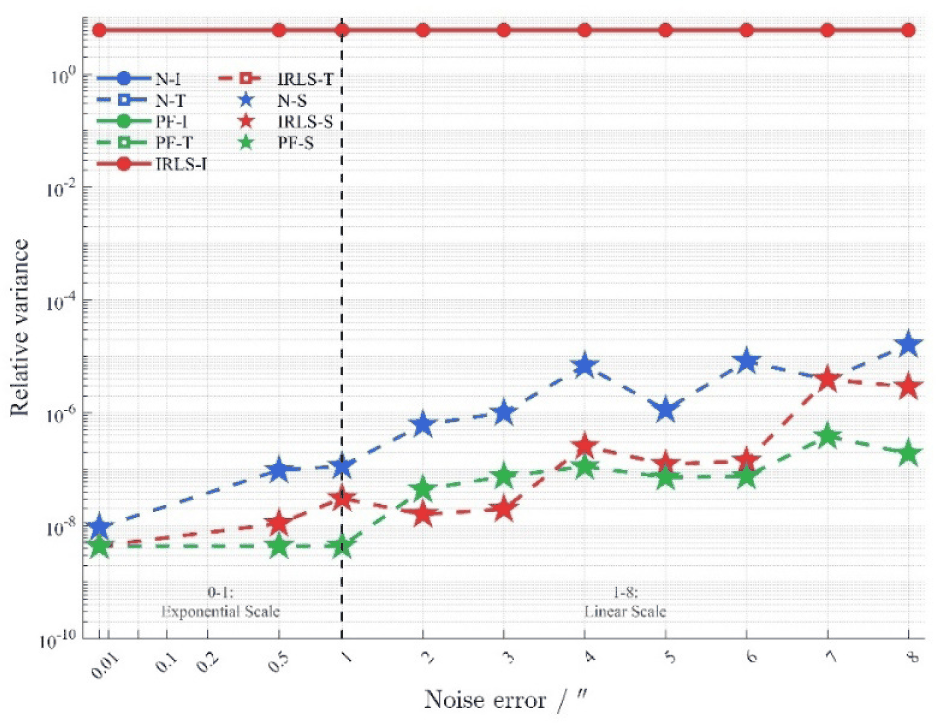
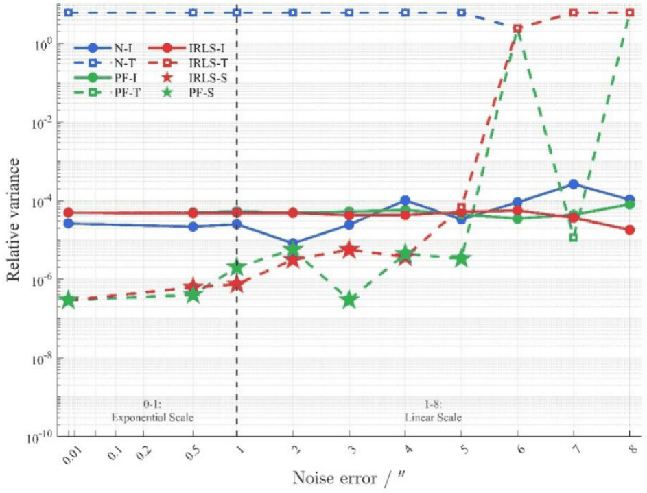
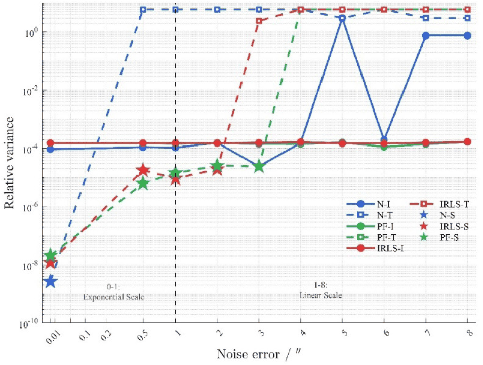
Analysis of the charts reveals that: across all orbit types and noise levels, both polynomial fitting and IRLS methods significantly reduce the relative variance of both correct and erroneous solutions, with the relative variance of correct solutions generally lower than that of erroneous solutions. Especially when noise ≥ 3″, the relative variance of correct solutions under the polynomial fitting method remains stable, while that of erroneous solutions increases significantly, creating a clear distinction. This indicates that the preprocessing method of this paper not only effectively smooths observation noise and eliminates gross errors but also enhances the discriminability of the solution sets, providing a reliable basis for subsequent erroneous solution elimination based on relative variance. Overall, the polynomial fitting method, while ensuring computational efficiency, achieves noise reduction and solution set separation effects similar to the IRLS method, and is therefore selected as the preprocessing method in this paper.
Addressing the erroneous solution problem in the AR algorithm for space-based angle-only initial orbit determination, this paper proposes an improved calculation method incorporating data preprocessing. The core idea of the algorithm is to distinguish between true and erroneous solutions based on the difference in stability of solution results under different geometric configurations after preprocessing the observation data. A pseudo-code description of the complete calculation flow of this method is shown in Algorithm (Fig. 9).
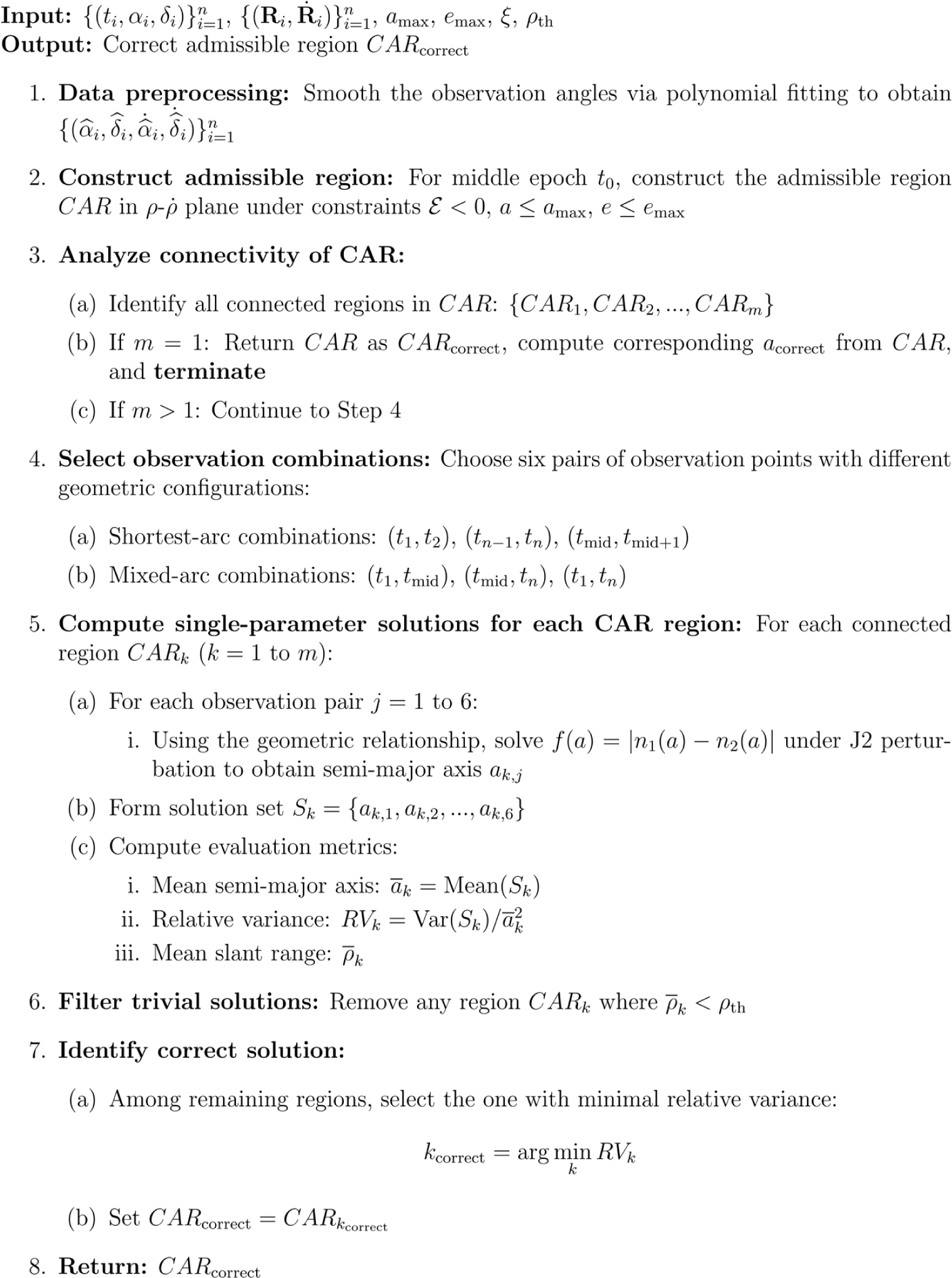
This flow enhances the quality of input data through a front-end data preprocessing module. Subsequently, the multi-geometry-configuration solution strategy amplifies the difference in statistical stability between true and erroneous solutions. Finally, through dual-threshold criteria based on relative variance and slant range, effective elimination of erroneous and trivial solutions is achieved. This method systematically integrates observation data purification, multi-solution path exploration, and statistical decision-making, significantly improving the reliability and robustness of space-based near-circular orbit initial orbit determination.
3. SIMULATION EXPERIMENTS AND RESULTS ANALYSIS
To comprehensively evaluate the erroneous solution suppression capability, orbit determination accuracy, and algorithm robustness of the proposed RV-SPSS method for space-based angle-only initial orbit determination, this chapter designs simulation experiments for two different scenarios. The first set of experiments employs high-fidelity simulations based on real TLEs and precise historical orbit data, focusing on verifying the algorithms performance under observation accuracy close to real conditions. The second set of experiments uses large-scale random orbit simulations to examine the algorithms robustness and broad applicability under typical low-Earth orbit observation platform configurations. All experiments use the success rate and error of semi-major axis (SMA) determination as the core evaluation metrics.
This set of experiments aims to construct a high-precision, highly realistic simulated observation environment to verify the core capability of the RV-SPSS method to identify and eliminate erroneous solutions under complex, near-actual working conditions. The data generation follows the process below: First, 50 LEO objects with continuous ground-based photoelectric observation data between January and June 2023 are selected. Their historical TLEs are used as initial orbits, and corresponding ground-based angle measurement data are used for precise orbit determination and prediction, generating high-precision orbital ephemerides (position accuracy better than 10 m) within the reference period. This study sets the space-based observation platform in LEO orbit, as it can perform wide-area surveillance of medium and high-altitude objects and is more likely to obtain very-short-arc observation data for a large number of space objects. This configuration aligns with the survey mission mode of space-based space surveillance, and existing research indicates that LEO observation platforms have advantages in associating multi-object observation data (Fujimoto & Scheeres 2013). This scenario can effectively validate the erroneous solution suppression capability of the proposed algorithm in surveillance mode. Subsequently, the SWARM satellite, which has global observation data and laser ranging support, is selected as the simulated space-based platform to generate high-precision platform orbits (orbit determination root mean square (RMS) ~0.7 m) for the same period. Finally, the precise ephemerides of the object and platform are differenced to calculate the objects right ascension and declination observation sequence relative to the platform. Gaussian white noise with zero mean and a standard deviation of 2 arcseconds is added to simulate measurement errors. This value is chosen to be representative of the typical accuracy of space-based optical sensors, which is reported to be in the range of 0.8–1.5 arcseconds for modern star trackers (Agostinelli et al. 2024).
The orbit extrapolation and precise orbit determination processes employed high-fidelity dynamic models; specific parameter settings are shown in Table 3. Furthermore, the simulation set the arc length to 80 s. Fig. 10 shows the parameter information for the simulated arcs. It should be noted that although actual space-based optical observation is also subject to various constraints such as Earth shadow, solar stray light, and camera field of view, these factors primarily affect object visibility and data quality and have a minor impact on the observation geometry and erroneous solution generation mechanism central to this study; therefore, they were not included in the simulation.
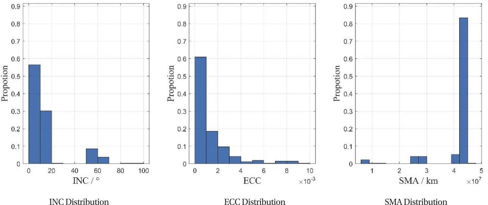
To test the algorithms applicability and erroneous solution suppression capability across different orbital configurations, this set of experiments constructs a large-scale random simulation scenario. The observation platform is set in a typical near-circular Low Earth Orbit. Object orbits are randomly generated for 300 space objects based on the parameter ranges for LEO, MEO, and GEO objects in Table 4, ensuring that objects are not occulted by Earth relative to the platform and are within the preset field of view during the simulation period. Based on two-body dynamics considering J2 perturbation, numerical integration generates precise orbits for objects and platforms, from which noise-free angle observation sequences are calculated. Finally, the measurement noise is modeled as zero-mean Gaussian white noise with a standard deviation of 2 arcseconds. The observation arc length is set to 80 s. This scenario aims to systematically verify the broad effectiveness and stability of the erroneous solution exclusion mechanism of the RV-SPSS method when facing a large number of randomly generated orbital objects and different observation arcs.
To quantitatively evaluate algorithm performance, we define three core metrics: Erroneous Solution Avoidance Success Rate—the proportion of cases where the algorithm successfully identifies and eliminates erroneous solutions, resulting in the final output being the correct solution among those containing erroneous solutions; and Semi-Major Axis Error Distribution—the percentages of correct solutions with absolute semi-major axis errors below 100 and 200 km. The proposed RV-SPSS method is compared with the baseline Admissible Region-Single Parameter (AR-SP) method. The AR-SP method operates by uniformly sampling the admissible region (constructed from energy, semi-major axis, and eccentricity constraints as described in Section 2.2) and, for each sampled (ρ, ) point, applying the single-parameter method (Section 2.3.2) to compute the corresponding orbital semi-major axis. The final output is the arithmetic mean of all these semi-major axis values. This approach represents the direct application of the single-parameter method without any mechanism to discriminate between true and erroneous solutions.
Fig. 11 shows a scatter plot of the solution set distribution based on TLE-derived data. The horizontal axis represents the mean of the solution sets SMA, and the vertical axis represents the solution sets RV. The plot distinguishes three cases: “Correct Solution,” “Erroneous Solution,” and “Large-Error Solution.” “Correct Solution” refers to the solution with SMA error < 200 km and the smallest relative variance; “Erroneous Solution” refers to solutions that are not the one with the smallest relative variance; “Large-Error Solution” refers to the solution that, although having the smallest relative variance, is not the one with the smallest error.
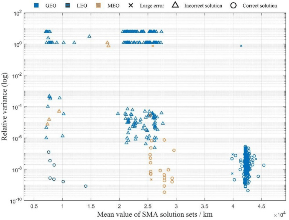
It can be seen from the figure that erroneous solutions and large-error solutions are more dispersed in the relative variance-semi-major axis plane, while correct solutions are relatively concentrated, verifying the insensitivity of the true solution to observation geometric configurations. Among a total of 269 observation arcs, 239 exhibited erroneous solutions, accounting for approximately 88.8%.
Table 5 compares the performance of different IOD methods on TLE-derived data, including the original AR-based single-parameter method, the proposed RV-SPSS method, as well as the Gooding and improved Gooding (I-Gooding) methods (Yin et al. 2023). While the I-Gooding method shows improvement over the original Gooding method, both algorithms demonstrate limited performance in the test scenarios which include a mix of LEO, MEO, and GEO objects. Gooding-based methods are known to be sensitive to measurement errors, and their orbital constraint effectiveness diminishes for MEO and GEO objects over short observation arcs, leading to degraded stability. In our statistical analysis, the probability of large errors (SMA error > 500 km, as a proportion of errors > 200 km) for the Gooding and I-Gooding methods reached 90.9% and 88.0%, respectively. In contrast, the erroneous solution convergence ratio for the original AR method was 88.8%. The proposed RV-SPSS method, through multi-direction solution set variance screening and slant range threshold exclusion, drastically reduced this ratio to below 5.5%. Simultaneously, it increased the percentage of SMA errors less than 100 km from 69.1% to 80.0% and less than 200 km from 76.6% to 90.5%. These results demonstrate that the proposed method, by specifically targeting geometry-induced erroneous solutions, offers superior robustness and accuracy compared to both the original AR method and recent Gooding-based approaches in a space-based very-short-arc IOD context.
To evaluate the robustness of the proposed RV-SPSS method under more challenging observation conditions, we performed additional experiments with varying levels of measurement noise. Three additional noise levels (3″, 4″, and 6″) were tested, while keeping all other simulation parameters unchanged. The results are summarized in Table 5. It can be seen that the erroneous-solution convergence ratio remains below 7% for 3″ noise and below 20% even for 6″ noise, while the percentage of semi-major axis errors below 200 km stays above 87% for 3″ noise and above 69% for 6″ noise. These sensitivity tests confirm that the RV-SPSS algorithm maintains its effectiveness under degraded data quality, demonstrating its practical applicability in realistic space-based surveillance scenarios.
The experimental results clearly indicate that the erroneous solution problem in the AR algorithm for space-based observation is pervasive. As shown in Table 6, without erroneous solution suppression measures, the AR algorithms convergence ratios to erroneous solutions in random simulation experiments for LEO, MEO, and GEO objects were 52.8%, 64.6%, and 17.7%, respectively. This data confirms that even for objects with randomly distributed orbital parameters, due to the complex relative motion geometry between the space-based observation platform and the objects, the generation of mathematically valid but physically unrealistic erroneous solutions by the AR algorithm under angle-only observation conditions is a frequent occurrence, particularly more prominent in MEO and LEO orbit scenarios.
| Method | Covergence to incoreect solutions-LEO (%) | Covergence to incoreect solutions-MEO (%) | Covergence to incoreect solutions-GEO (%) |
|---|---|---|---|
| AR | 52.8 | 64.6 | 17.7 |
| The proposed method | 5.5 | 2.0 | 5.4 |
Further analysis of the distribution of erroneous solutions, as illustrated in Fig. 12 using large-scale random orbit simulations (300 objects across LEO, MEO, and GEO), provides direct experimental validation of the core theoretical principle established in Section 2.3—namely, that true solutions are invariant under geometric variations, while erroneous solutions are highly sensitive to such changes. This theoretical distinction is clearly reflected in Fig. 12 from two perspectives. First, examining the horizontal axis (semi-major axis values), erroneous solutions are widely dispersed across a remarkably broad range, from below 10,000 km to over 46,000 km. This dispersion validates the theoretical prediction that erroneous solutions are geometry-dependent: different targets have inherently different observation geometries, and the resulting erroneous solutions therefore take on correspondingly different values. Even for GEO objects, whose orbital altitudes are relatively concentrated, erroneous solutions span an interval from 10,000 km to 46,000 km, demonstrating that these erroneous solutions cannot be eliminated by simple numerical constraints based on prior orbit type assumptions. Second, examining the vertical axis (relative variance of solution sets), correct solutions consistently cluster in the low relative variance region (below 10–6), demonstrating their stability across different geometric configurations. In contrast, erroneous solutions predominantly concentrate in the high relative variance region (above 10–5). This distribution directly validates two key theoretical claims: (1) the relative variance criterion serves as an effective discriminator for distinguishing true solutions from erroneous ones, and (2) erroneous solutions are indeed sensitive to changes in observation geometry, manifesting as high statistical dispersion when evaluated across different geometric configurations. Critically, these patterns hold consistently across LEO, MEO, and GEO objects in the large-scale random simulation, confirming that the theoretical principle—and the screening strategy based upon it—is broadly applicable rather than limited to specific orbital regimes.
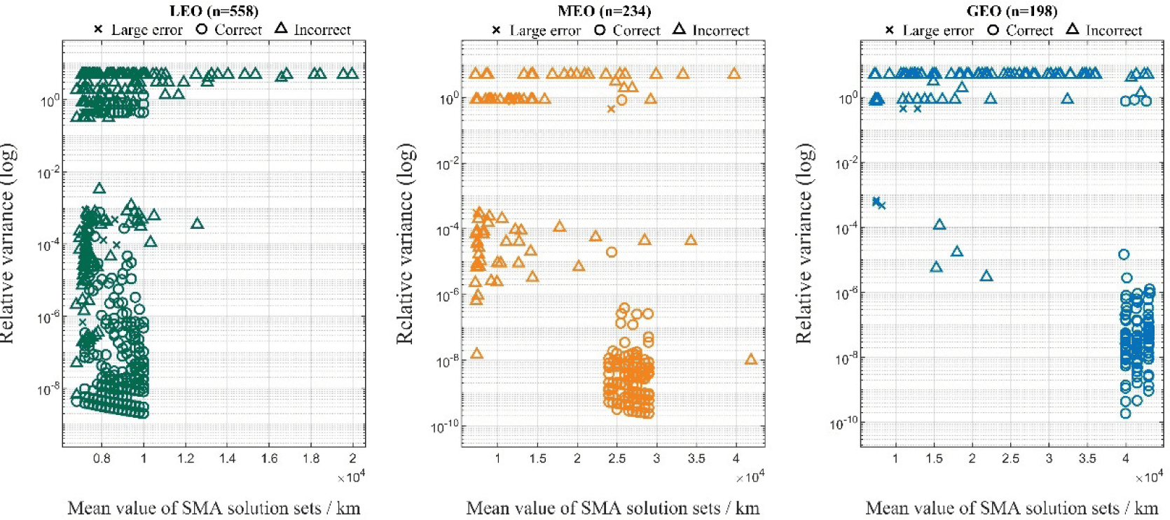
This inherent geometry-dependence of erroneous solutions means that relying solely on prior orbit type assumptions and setting numerical constraints is insufficient to effectively identify and eliminate them. Therefore, the RV-SPSS method proposed in this paper, by constructing multi-geometry-configuration solution sets and discriminating based on their statistical stability, provides a theoretically grounded and more effective approach to solving such erroneous solution screening problems.
The proposed RV-SPSS method demonstrated excellent erroneous solution suppression capability and algorithm robustness in the random simulation experiments. After applying this method, the erroneous solution convergence ratios for LEO, MEO, and GEO objects significantly decreased to 5.5%, 2.0%, and 5.4%, respectively. This improvement indicates that by constructing multi-geometry-configuration solution sets and using their relative variance for stability discrimination, erroneous solutions arising from changes in observation geometry can be effectively identified and eliminated. It is particularly noteworthy that the erroneous solution ratio for MEO objects drastically dropped from 64.6% to 2.0%, demonstrating the methods strong adaptability and robustness to the complex relative motion geometry in the medium Earth orbit region. Similarly, the method shows stable erroneous solution elimination effects for LEO and GEO objects, further verifying its wide applicability across different orbital altitudes and motion characteristics.
4. CONCLUSIONS
This paper addresses the erroneous solution problem in the initial orbit determination of near-circular orbits under space-based observation. It reveals the geometric causes of these erroneous solutions and proposes a suppression method based on stability analysis of multi-direction solution sets (RV-SPSS). This method constructs observation combinations with different geometric configurations and leverages the significant difference in statistical stability between true and erroneous solutions to effectively eliminate the latter. It also incorporates data preprocessing and a slant range threshold judgment to enhance robustness.
Simulation experiments validate the effectiveness of the proposed method. Experiments based on historical data show that the method reduces the proportion of erroneous solutions from 88.8% to below 5.5% and increases the proportion of semi-major axis errors less than 200 km to 90.5%. Large-scale random orbit simulations further confirm that the methods erroneous solution suppression rate remains stable within 6% for LEO, MEO, and GEO objects, demonstrating good general applicability.
This work provides a more reliable solution for space-based very-short-arc initial orbit determination. Future efforts will extend the method to orbits with larger eccentricities and promote its application to real observational data.

