Magnetometer Calibration Based on the CHAOS-7 Model

1. INTRODUCTION

A magnetometer that measures magnetic field vectors is essential for satellites going into space. It is used either as a navigation compass to determine the attitude of satellites in space, or as a tool to measure the Earth’s magnetic field changes and to study/monitor the space environment around the Earth. A Flux Gate Magnetometer (FGM) generally has three axes, which can measure both the magnitude and direction of magnetic field vectors. On the other hand, a scalar magnetometer can only measure the magnitude of geomagnetic fields, but with a high degree of precision. An FGM that is sensitive enough to measure weak changes of Earth’s magnetic field at the nanotesla level is an indispensable scientific payload for satellites monitoring the space environment. Previous observations of the Earth’s magnetic field on low Earth orbit (LEO) include Magsat, Ørsted, SAC-C, CHAMP, and Swarm (Olsen et al. 2014;Alken et al. 2020). The geomagnetic measurement data of these satellites was used to create CHAOS-7, the latest in a series of time-dependent geomagnetic field models developed at Denmark Technical University (DTU) (Olsen et al. 2003, 2014;Finlay et al. 2020). The CHAOS models and the precise geomagnetic data utilized for their construction have been widely used in scientific studies, and now can also be applied to magnetometer calibration (Olsen et al. 2020). The CHAOS-7 model has higher spherical harmonics degrees then the IGRF-13, which allows for more detailed variations of the Earth’s geomagnetic field (Alken et al. 2020;Finlay et al. 2020). In addition, CHAOS-7 provides regular updates, typically every four to six months, using the latest satellite and ground data (Finlay et al. 2020).

In general, pre-flight calibration involves a large amount of ground-based experiments before launch (Connerney et al. 2017). The purpose of pre-flight calibration is to ensure that the instrument will measure components of the natural magnetic field correctly in scientific units such as the International System of Units (SI), and maintain this capability throughout the mission in space (Risbo et al. 2003). It mainly characterizes temperature dependences, non-orthogonality, and noise levels around the FGM, such as magnetic disturbances by currents flowing in the onboard electronic devices. Unlike the pre-flight calibration, the CHAOS-7 model can be used for in-orbit (post-launch) calibration, e.g., periodic re-calculation of calibration parameters based on the data downloaded from space.

In this paper, we describe the process of obtaining the calibration parameters of FGM through comparison of the data with the CHAOS-7 geomagnetic field model. The code is designed to find the calibration parameters autonomously by mapping the FGM data to the corresponding CHAOS outputs. For performance evaluation, the differences between the prescribed and reconstructed calibration parameters are investigated before we apply the method to real satellite observation data. Model outputs and satellite data have different coordinate systems, so they need to be transformed into the common star tracker coordinate (STC). The model output is first converted from an Earthfixed coordinate to a celestial coordinate system and then to the STC using the quaternion data of the star tracker, which represents the spacecraft’s attitude. The FGM data should be corrected with a set of calibration parameters to match the CHAOS-7 data in the STC. The parameters to be evaluated in this optimization process include the instrument gain, offset, non-orthogonality, and Euler’s rotation between the FGM frame and the STC. We demonstrate the performance of our code, which we plan to apply to actual satellite observations in the future. To validate the code’s performance, we first generate pseudo data by convoluting the ‘true’ CHAOS-7 data with prescribed instrument characteristics, which are the reverse calibration parameters. The parameter values are considered ‘true’ calibration parameters that should be pursued by our program autonomously. The program reconstructs the calibration parameters by comparing the pseudo data and the ‘true’ CHAOS-7 outputs. In the optimization process, we obtain the calibration parameters and finally compare them to the initially prescribed values for performance evaluation. All the processes are performed using Python 3.8.5, NumPy 1.19.2, SciPy 1.6, AstroPy 4.2, SpacePy 0.2.1, and ChaosmagPy 0.5 including the CHAOS-7.6 geomagnetic field model. In the future, this code will be used for in-orbit calibration of the magnetic field data from the NEXT generation small Satellite-1 (NEXTSat-1) operated by the Satellite Technology Research Center (SaTReC) of the Korea Advanced Institute of Science and Technology (KAIST) (Kim et al. 2020), and from the Korea Astronomy and Space Science Institute Satellite (KASISat) of the Small scale magNetospheric and Ionospheric Plasma Experiment (SNIPE) mission under development at the Korea Astronomy and Space Science Institute (KASI) (Sohn et al. 2018;Kang et al. 2020).

2. COORDINATE TRANSFORMATION

The CHAOS-7 data and the satellite FGM data have different coordinate systems. The CHAOS-7 data are given in the local orthogonal coordinate system on spherical surfaces, consisting of the magnetic field components in the radius, theta, and phi directions (B_radius, B_theta, and B_phi), respectively in the local Up-South-East directions. The satellite magnetometer data has a coordinate system fixed to the satellite body. To compare these two data in the same coordinate system, we choose the orthogonal STC as the reference frame, because both CHAOS-7 and FGM data are easy to transform into the STC (Olsen et al. 2020). In the case of the CHAOS-7 output data, it can be converted to a celestial coordinate system via the local horizontal elevation-azimuth coordinate system, and then converted to STC using the quaternion data. To accomplish this, satellites must have sensors that produce quaternion attitude data, such as star trackers. On the other hand, the coordinate system of the satellite magnetometer data is fixed to the satellite's body along with the STC, so is possible to convert to STC using the Euler rotation matrix. This allows STC to compare the two data from different coordinate systems in a single frame.

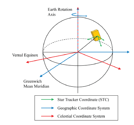
Fig. 1 shows three steps for transforming the CHAOS model outputs to STC. The green coordinate is the STC, which represents the coordinate system of the satellite body. The center of the STC is not the center of the earth, but the center of the star tracker fixed to the satellite body. The blue coordinate is the Earth-fixed geographic coordinate known as the Earth Centered Earth fixed (ECEF) coordinate, used to determine the satellite’s location in longitude and latitude, and the x-axis points to the Greenwich meridian, so the whole frame rotates with the Earth. The red coordinate system is the celestial coordinate system at the center of the earth, and the x-axis indicates the vernal (March) equinox. The CHAOS model outputs given in the local up-south-east coordinate at the satellite location, which is interlocked with the Earth-fixed geographic coordinate (Blue), are first transformed to the celestial coordinate (Red) via SpacePy and AstroPy. We further transform the vectors from the celestial coordinates to STC (green) with the quaternion data of the star tracker.

Fig. 1. Geographic, Celestial, and Star Tracker Coordinates for the magnetometer calibration.

Download Original Figure

3. PARAMETERS

Satellite observations of the geomagnetic field are initially in the FGM frame, which is inherently non-orthogonal due to manufacturing errors, thermal distortion of mechanical structures, etc. In addition, the real-world FGM may have nonzero offsets and non-unity gains. Therefore, in this paper, we use four matrices in total to describe those nonideal effects: b, R, S, and P. The 4 matrices in turn consist of 21 calibration parameters: 9 at b, 6 at S, 3 at P, 3 at R matrices, as shown in Table 1.

Table 1. Characterization Parameters for the FGM calibration

Download Excel Table

By the calibration process described below, the raw FGM data (B_FGM) are calibrated and converted to STC. B_CHAOS is the CHAOS-7 outputs data in STC by the coordinate transformation process, and can be related to the natural geomagnetic field as

where B_FGM is the FGM data in the non-orthogonal FGM coordinate (Olsen et al. 2020). In Eq. (1), the element values of matrix S, P, R, and b are to be evaluated by the optimization process.

is the offsets for the three axes (arms) in nT.

is the scale (or gain) values as a diagonal matrix.

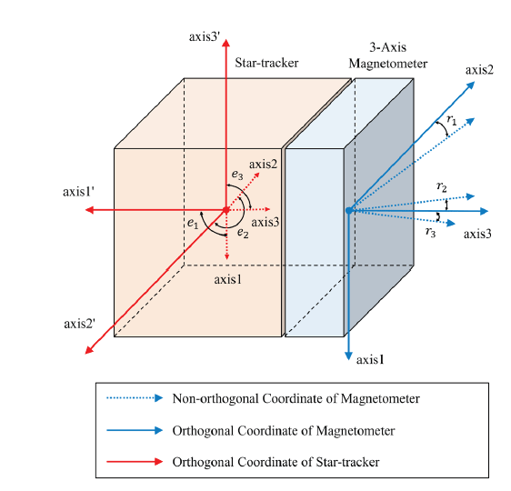
is the non-orthogonality matrix which transforms magnetic field vectors from the ideal orthogonal frame to the nonorthogonal FGM frame. The former and the latter frames share one common axis, which is assumed to be the x-axis of the FGM without loss of generality. The r₁, r₂, and r₃ are angles representing the non-orthogonality of FGM.

is the Euler rotation matrix from the STC coordinate to the orthogonalized FGM frame.

In place of real satellite FGM data for comparison with the CHAOS model, we generate pseudo data of FGM and use them to demonstrate the performance of our code. The pseudo data (B_{FGM_PSEUDO}) is produced by distorting the CHAOS model outputs (B_CHAOS), which is first transformed to STC in the opposite order (Eq. (6)) of the optimization (Eq. (1)). The values of the parameters used in this distortion process as Eq. (6) are considered the “true” parameter values, which should be found by optimization.

Fig. 2 describes the non-orthogonality matrix P(r) and the Euler rotation matrix R(e). The blue dotted arrow is the nonorthogonal coordinate of the magnetometer, and needs to be aligned to a blue solid arrow which is the orthogonalized coordinate of the magnetometer. For non-orthogonality correction, magnetometer axis1 is assumed to be projection invariant, axis2 has a single degree of freedom in the axis1–2 plane, and axis3 has two degrees of freedom. The three degrees of freedom are represented by r₁, r₂, and r₃ as three angles (Merayo et al. 2001;Olsen et al. 2003). The red coordinate is the orthogonal STC. To rotate from the STC to the orthogonal FGM coordinate, the Euler rotation matrix R is used with parameters e₁, e₂, and e₃.

Fig. 2. Elements of the non-orthogonalities (r₁, r₂, r₃) and the Euler rotation angles (e₁, e₂, e₃) on the star tracker and the magnetometer.

Download Original Figure

4. OPTIMIZATION

The CHAOS model outputs are the reference data for this research. Input data for the CHAOS model include time, latitude, longitude, and altitude. We assume 1 Hz sampling rate of the FGM and generate CHAOS model outputs at 10,800 points for 3 hours, from 2020/03/21 00:00:00 to 2020/03/21 03:00:00 in universal time. The geographic latitude range is from –80 to 80 degrees, the longitude range is from –160 to 160 degrees, and the altitude is constant at 500 km.

T is the temperature of the magnetometer, and I is the electric current flowing around the magnetometer, both of which should be provided by the spacecraft telemetry data. In this paper, we use pseudo telemetry of the temperature (T) which is a time series in the form of sine function between –120℃ and 120℃, and pseudo telemetry of current (I) as a sine function between 0 A and 1 A. In addition, the quaternion data simply assume a constant of [0, 0.707, 0, 0.707] in the form [x, y, z, w].

The 21 calibration parameters are tracked down by optimization processes based on the ‘scipy.optimize.least_ squares’ function of the SciPy module. The least squares function solves a nonlinear least-squares problem with bounds on the variables. The method used in this study is the ‘trf ’ (Trust Region Reflective) algorithm, which is particularly suitable for large sparse problems with bounds. The cost function is a sum of squares of the vector residuals between B_optimized and B_CHAOS in STC, and becomes zero when B_optimized = B_CHAOS. B_optimized is the FGM data calibrated by the optimum calibration parameters corresponding to the minimum cost function.

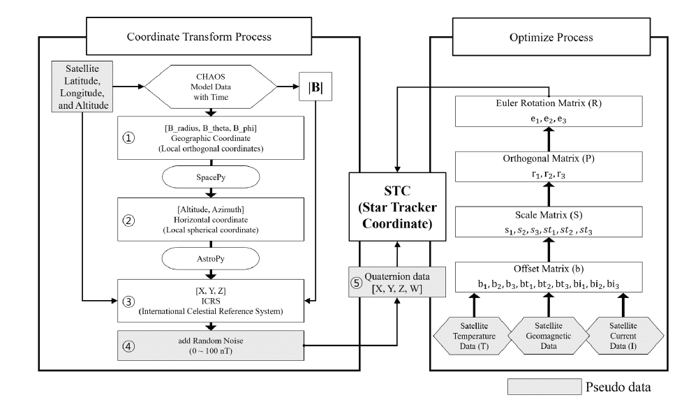
The purpose of the optimization process is to find the optimal values of the 21 unknown calibration parameters. Fig. 3 presents the flow chart of the process consisting of coordinate transformation and optimization. At the center of Fig. 3 is the STC, to which both the CHAOS model and FGM observation data should be transformed. The coordinate transformation process on the left side of the Fig. 3 describes the sequence in which the CHAOS model outputs are transformed to the STC frame. The process on the right of Fig. 3 uses calibration parameters to post-process the satellite data and to transforms the results to STC.

Fig. 3. Process diagram for in-orbit magnetometer calibration.

Download Original Figure

Steps 1-4 below represent the process of generating ‘true’ magnetic field predicted by the CHAOS model and transforming it to the STC. Steps 5–6 describe processes for recovering the prescribed calibration parameters by the non-linear optimization between the pseudo data and ‘true’ CHAOS model outputs.

5. RESULT

The result of the optimization is shown in Fig. 4. The red circles are the originally prescribed calibration parameter values which are used to generate pseudo data by distorting the ‘true’ CHAOS model. The blue stars are the values reconstructed by the optimization, which are the products of the calibration process expressed to the right of Fig. 3. The yellow diamond shapes are the initial seed values given at the beginning of the nonlinear optimization, and the black triangles are the lower and upper bounds, which serve as the minimum and maximum limit of the parameter range from which the result should be obtained. The closer the blue stars representing the optimization results are to the red circles representing the true value, the more accurate the optimization. Therefore, within the 3-hour time range of the pseudo data, the 21 “basic” calibration parameters (9 offsets, 6 scale values, 3 non-orthogonalities, and 3 Euler angles) can be reconstructed, and the results prove to be very close to the originally prescribed values (red circle). Fig. 4 demonstrates that our code can find the parameters in the upper row (S, P, and R matrices) more accurately than the offsets (b matrix) in the lower row.

Fig. 4. Parameter comparison between the true values and the optimized values with 100 nT of noise.

Download Original Figure

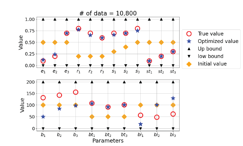
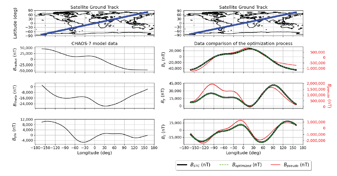
Fig. 5 presents the pseudo FGM data, reconstructed magnetic field based on the optimized calibration parameters, along with the ‘true’ (STC-converted) data of the CHAOS model outputs. Each column has the same x-axis scale. The graphs in the top row represent satellite trajectories on a world map, which are set up to create the pseudo data. The three graphs in the left column are the ‘true’ magnetic field from the CHAOS model, showing the magnetic field values at the pseudo satellite location in the local orthogonal Radius (radially up), Theta (geographic south), and Phi (geographic east) directions. The graphs in the second-to-fourth row of the right column represent the true CHAOS output in the STC (right column, black curves), the raw pseudo data (right column, red curves), and the calibrated magnetic field through the optimized 21 calibration parameters (right column, green dots). As is naturally expected, the ‘true’ CHAOS model outputs (black curves) match better with the calibrated data by the 21 calibration parameters (green dots) than with the raw pseudo data (red curves). The black scales on the left y-axis are for the ‘true’ CHAOS model outputs (black curves) and the calibrated data (green dots), and the red scale on the right y-axis is for the raw pseudo data (red curves).

Fig. 5. (top) Ground track of the pseudo FGM data, (left) CHAOS model outputs in the local orthogonal frame, and (right) the pseudo FGM data, the reconstructed magnetic field based on the optimized calibration parameters, along with the ‘true’ (STC-converted) model outputs. STC, star tracker coordinate.

Download Original Figure

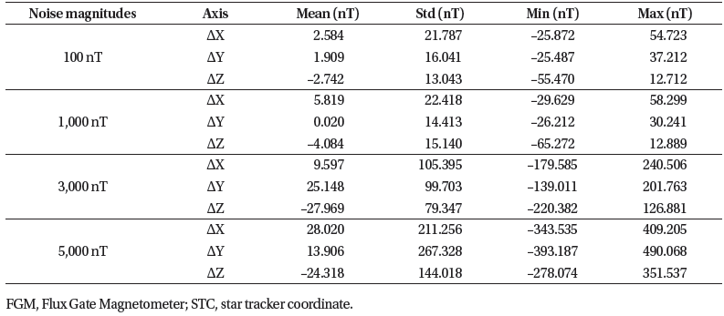
Although there is a nonzero difference between the optimization value and the true value of the parameters, the pseudo-data calibrated by the optimum parameters is quite similar to the CHAOS data. Table 2 shows the distribution of the quantitative differences by each axis; Mean, Standard deviation, Minimum, and Maximum values. In addition, we have repeated the optimization process with stronger instrument noise (i.e., 1,000 nT, 3,000 nT, and 5,000 nT instead of the 100 nT previously used). According to the values given in Table 2, our code works well up to the noise level of 1,000 nT. However, at noise levels exceeding 1,000 nT, the code has difficulty in finding the appropriate calibration parameters: increasing the noise magnitudes results in a greater error. That is, our code can reconstruct the true magnetic field when the instrument noise level is within 1,000 nT.

Table 2. Statistics of difference between the CHAOS-7 data and the calibrated FGM data in STC

Download Excel Table

6. DISCUSSION

According to Olsen et al. (2003), in addition to the basic parameters, we may include parameters representing magnetorquer coupling and sensor cross‑talk. Also, we may use separate parameters for solar panel and battery currents. For simplicity, the magnetorquer coupling and sensor cross‑talk are not considered in this preliminary study, and various onboard currents affecting the magnetometer were also treated as one parameter. While only the basic parameters were estimated here, the results in Section 5 demonstrate that our simplistic approach and the resultant code perform reasonably well.

In the future, the basic calibration parameters will be obtained in a more realistic environment, e.g., based on actual observation data from the lately launched Next Generation Small Satellite-1. After that, the code can also be used to calibrate the magnetometer of the SNIPE satellite, which is scheduled to be launched later in 2021. Progressively, not only the basic parameters but also other parameters like cross-talk will be obtained through optimization, so that values much closer to the natural magnetic field can be reconstructed.

7. CONCLUSION

A magnetometer, which is an essential payload for satellites, measures magnetic fields and is used for the attitude determination of the satellite or for scientific research such as the geomagnetism and space weather. Because the magnetometer is inherently sensitive to ambient temperature and current as well as manufacturing errors, calibration should be performed periodically. For in-orbit calibrations of FGM in the absence of an absolute scalar magnetometer, geomagnetic field models are indispensable.

We address a method for in-orbit calibration of bodymounted magnetometers based on the CHAOS-7 geomagnetic field model. To compare the CHAOS-7 model outputs with the magnetometer measurement data, a common coordinate system is required. The common coordinate system is set to the frame of the star tracker, because quaternion data from the star tracker transform vectors from the Earth-fixed to the star tracker frame via celestial coordinates. The parameters to be found in the optimization process are gain, offset, orthogonality, and Euler rotation, with 21 basic parameters in total. After we generate pseudo data by distorting the ‘true’ CHAOS-7 data using prescribed calibration parameters, we let the python code autonomously track down the parameters through optimization processes.

In conclusion, given the initial value, the upper limit, and the lower limit of the nonlinear optimization, the basic parameters close to the true values can be reconstructed. The agreement confirms the accuracy of our optimization code. In addition, we compare the true model outputs with the pseudo data calibrated by the ‘tracked down’ parameters, and observe a high degree of similarity. The optimization result of the offset (b) is not as accurate as the other calibration parameters, such as S, P(r), and R(e). However, the magnitudes of those offsets (several tens of nanoteslas) are generally much smaller than the geomagnetic field intensity. The limited performance of the offset retrieval does not severely compromise the overall calibration performance, as long as the S, P(r), and R(e) parameters are properly tracked down.