1. INTRODUCTION
Korea has launched more than 20 satellites including CubeSats, and is therefore required to monitor satellites and provide information. The Korea astronomy and space science institute (KASI) developed the first electro-optical monitoring system, optical wide-field patrol network (OWL-Net) and has operated to acquire optical images and extract tracking data from the images independently (Park et al. 2013). Optical observations include not only common errors such as observational noise and bias, but also the errors caused by clock accuracy or optical equipment characteristics such as the reflection of the light in the mirror of the telescope, the difference between the speed of the computer and the CCD camera, mismatch of the background stars between the star list and the image, and the shutter speed of the CCD camera. Therefore, an algorithm which estimates the orbit by correcting various errors is needed to calculate the orbital information of the satellite using the optical observation data.
In this study, precise orbit determination (POD) software that can independently determine satellite orbits with optical observation was developed, verified, and validated. The POD system consists of a dynamic model, a measurement model, and an estimation algorithm. The dynamic model contains perturbations of the Earth gravitational field, atmospheric drag, solar radiation pressure, and solar/lunar gravity. To verify the dynamic model, a state vector was propagated for 24 hours from the same epoch time by both the general mission analysis tool (GMAT) and the dynamic model developed, and the trajectories were compared to each other. The measurement model provides topocentric right ascension (RA) and declination (DEC), and error models of light travel time, annual aberration, and diurnal aberration. It was verified by comparing the observations from the model to that printed out by GMAT. In the case of the estimation algorithms, two types of batch filters were used—the least-squares (LS) batch filter and the unscented transform (UT) batch filter. Previously conducted studies on OWL-Net (Lee et al. 2017;Choi et al. 2018) used LS batch filter, including a linearization process, but it may cause a large error or divergence when the initial condition is inaccurate (Park et al. 2010). The UT batch filter, however, is a nonlinear filter that can overcome the disadvantages of linearization. To verify the POD software developed, artificial optical observation data were generated in GMAT, and POD was performed under the various initial conditions. Finally, the real optical observation data of low Earth orbit (LEO) satellite, Cryosat-2, observed by OWL-Net were employed to validate the software.
In section 2, the overall construction of the POD software is introduced and mathematically explained. The verification of each algorithm in the POD software is described in section 3, and validation using the actual observation data from OWL-Net is exhibited in section 4. Section 5 summarizes the paper.
2. PRECISE ORBIT DETERMINATION (POD)
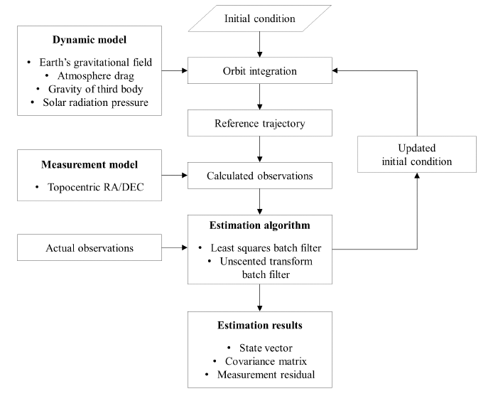
The purpose of satellite orbit determination (OD) is to obtain the satellite orbital elements in terms of the position and velocity vector at a specific time. The nonlinear system equation consists of forces affecting satellites, the measurement model, and an estimation algorithm. The OD process is conducted to minimize the measurement residual, the difference between actual observations and observations calculated through the system equations for estimating the orbit elements. Fig. 1 demonstrates the flowchart of the POD software developed in this study. If initial conditions are given, the reference trajectory is generated by propagating the orbit using a dynamic model, and the observations are computed using the measurement model. Then, iterative computation is performed until the convergence condition is satisfied, and then the orbit estimation result is calculated as a state vector, a covariance matrix, and a measurement residual. In this section, we mathematically describe the dynamic model, the measurement model, and the estimation algorithm reflected in the POD software.
A satellite moving near the Earth is affected by various forces, and the dynamic model mathematically describes the forces. In this study, the dynamic model was designed considering the perturbations caused by the Earth’s asymmetric gravitational field, the atmospheric drag, the solar radiation pressure, and the lunar/solar gravity (Vallado 2001). The dynamic model developed includes a JGM3 model for the Earth gravitational field, an exponential model for atmospheric density, and an analytical approximation for lunar/solar gravity. The Runge-Kutta 5th method is also employed for a numerical integrator. Note that the detailed equations are not presented in this section.
The optical observations are based on the topocentric equatorial coordinate system (ItJtKt), and the geometric relationship between the satellite and the ground station is illustrated in Fig. 2 (Vallado 2001). The ItJtKt coordinate system, which moves the center of the geocentric equatorial coordinate system (IJK) to the ground station, rotates with the Earth, but the axes are fixed. The and axes are parallel to the vernal equinox.
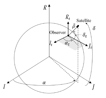
Satellites orbit around the Earth, and there is a difference between the geocentric and topocentric RA/DEC. When optical observations are performed, the topocentric RA/ DEC values (αt, δt) are extracted from the image. αt is the angle measured from the axis to the projected point after projecting the satellite on the ItJt plane, and δt is the angle measured from the point projected on the ItJt plane to the position of the satellite. The position vector of the satellite with respect to the ground station, is expressed as , where and are the position vectors in the geocentric equatorial coordinate system of the satellite and the ground station, respectively. If the components of in the It JtKt coordinate system are represented by (ρI, ρJ, ρK), the observations (αt, δt) are expressed as Eq. (1) by Fig. 2.
There are several errors affecting observation data due to the characteristics of optical observations such as light travel time, annual aberration, and diurnal aberration. These errors must be corrected because they could cause several tens of arcsec error in the case of LEO, hence correction models were developed for each error.
As the light speed is finite, a delay occurs by the light travel time from the observed object to the observatory. That is, when the position of the object is estimated using the observation data at the time t, the position of the object is not at the time t but t–τ where τ is the light travel time.
Annual aberration is a phenomenon caused by the movement of the earth’s observer by the Earth revolving around the sun. Because the Earth revolves in an elliptical orbit and the velocity changes periodically, the aberration also changes periodically. The aberration constant κ ′ , which means the maximum displacement of the observed object due to the annual aberration, is 20.4960”. The variations of RA/DEC due to the annual aberration, ΔRAA and ΔDECA, are given by Eq. (2) (Smart & Green 1977).
where λ is geocentric longitude of the sun in the ecliptic plane and ϵT is ecliptic inclination.
Diurnal aberration is a phenomenon caused by the velocity of an observer on the surface of the Earth as the Earth rotates. Therefore, it is influenced not only by the observational time but also by the latitude of the observatory. The effect of the diurnal aberration is 1/100 times that of the annual aberration, and the effect is the largest in the equator due to the fastest rotating speed. The diurnal aberration constant is defined as k = cosϕ where ϕ is the latitude of the observatory, and the variation of RA/DEC due to the diurnal aberration is given by Eq. (3) (Smart & Green 1977).
where h is an hour angle, obtained by subtracting RA of object from the local sidereal time.
The use of estimation algorithms can be classified as a batch processing method or a real time processing method. Because both the observation and the OD are performed on the ground, the batch processing method is primarily used for the optical monitoring system, in which observed values are extracted through data processing after the observation images are acquired. The batch estimation algorithm, or batch filter, is the OD technique that estimates a state vector at the epoch time after performing iterative calculation using a set of observed data acquired over a certain period.
The LS batch filter which is used generally includes a process of linearizing a nonlinear system. Thus, there is a disadvantage that if the initial guess value is not correct or the observed data is insufficient, it is possible to occur large estimation error or even divergence (Lee & Alfriend 2007). To overcome these drawbacks, a batch filter based on the UT has been devised (Park et al. 2010). The UT performs nonlinear transformation by generating 2L +1 points based on the probability distribution, where L is the dimension of the estimated state vector. Unlike the LS batch filter, there is no linearization process and therefore it is not sensitive to initial guesses (Park et al. 2010). In this study, a scaled UT method is employed for the nonlinear transform. Three scaling parameters, α, β, and κ, are required. α is an index indicating the range over which the sample is distributed, and β and κ are parameters for calculating the weight of the sample and the covariance matrix. κ is given by κ = 3 – L (Grewal & Andrews 2008). The sigma point generated based on the state vector Xk using the initial covariance matrix Pinitial is defined as Eq. (4) (Haykin 2001),
where λ is a parameter calculated by the scaling parameter and can be expressed by Eq. (5) (Grewal & Andrews 2008).
By introducing these UT techniques into a batch filter, the UT batch filter has been developed (Park et al. 2009;Park et al. 2010). In the batch filter, because the state vector at the epoch time is estimated using all observational data of a certain period, it is not necessary to propagate the state vector and the covariance matrix at any times except for the epoch time. Therefore, the sigma point, the state vector, and the covariance matrix at a particular time tk(χi,k, Xk, and Pk respectively) are the same as the estimated values (; Eq. (6); Park et al. 2010).
After the sigma points are generated at the epoch time, they are propagated to each observational time by the dynamic model F, and the calculated observations at each time can be obtained using the measurement model function h, expressed by Eq. (7) and (8), respectively.
In these equations, y is a computed observation for sigma points, and subscript k means a time tk (k = 1, ..., N) where N means the total number of observation data. The nonlinear computed observation Y is a weighted sum of y.
where is a weight factor for each sigma point.
Therefore, the estimated state vector at the epoch time is updated by (Park 2009).
where ΔZi is the O-C residual matrix, the subtracting the calculated measurement (Yi) from the actual measurement ( Y ) (Park et al. 2010) and Ki is the gain matrix defined as Eq. (11)
where is the covariance of observation matrix and is the cross-correlation matrix of the state vector and the calculated observations. Note that the superscription indicates the number of iterations because the algorithm is iterated until the convergence criterion is satisfied. The condition for terminating the iteration is given by
where RMS is root mean square, W is the weight matrix, n is the number of different types of observations, N is the total number of measurements, and ϵ is the value of convergence criterion (Vallado 2001).
3. VERIFICATION OF ALGORITHMS
In this section, the POD software developed in the MATLAB environment was verified against GMAT. GMAT is a space mission design software which has been validated and verified with almost 12,000 test cases for the script engine and almost 3,400 test cases for the graphical user interface (Hughes et al. 2014). The dynamic model was verified by comparing the trajectories propagated by the developed code and GMAT, and the measurement model was verified by analyzing the OWL-Net measurement residuals computed by the consolidated prediction format (CPF) provided by the international laser ranging service (ILRS; Pearlman et al. 2002). Both LS and UT estimation algorithms were verified through the simulation analysis using artificial observational data generated with GMAT.
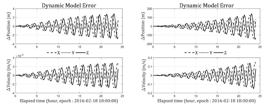
In order to verify the dynamic model, a state vector ( =[–4,981.8931, 842.9225, 5,118.8623] km, =[–4.8963, 2.2328, –5.1458] km/s) was propagated using MATLAB and GMAT for 24 hours from the epoch time (February 18, 2016, 18:00:00) with 10 min intervals. In the simulation environment of MATLAB and GMAT, the Earth gravitational field model (JGM3 10 × 10), the atmospheric drag coefficients (2.2), the solar radiation pressure coefficient (1.8), and the integrator (Runge-Kutta 5th with an accuracy of 10–9) were set equally. However, the atmospheric drag model (exponential model in MATLAB, and Jacchia Roberts in GMAT) and the lunar/solar gravity (analytic approximation in MATLAB, and DE421 in GMAT) were set differently because there is no identical model in both software. JGM3 10 × 10 was also chosen because 70 × 70 had a propagation position error of 0.5 m for 24 hours, but the calculation took nearly twice as long. To verify the performance of the developed propagator, the propagation error was checked by considering only the gravitational field, and then all perturbations, including the atmospheric drag, solar radiation pressure, and the lunar/ solar gravity. The left and right plots of Fig. 3 show the error over 24 hours when propagating the state vector considering only the Earth gravitational field model and all perturbations, respectively. Due to the position error being within 3 m and the speed error being within 0.003 m/s for the gravity only case, the performance of the JGM3 model was verified. Considering all perturbations, however, the position error was increased up to 100 m and the speed error was increased to 0.15 m/s. The difference was caused because the employed air drag model and exponential model is a simple and static model with low accuracy, while the Jacchia Roberts model, embedded in the GMAT, reflects various phenomena, such as variation of the Earth magnetic field and hydrogen density at high altitudes (Vallado 2001). Thus, the performance of the propagator developed in MATLAB was verified.
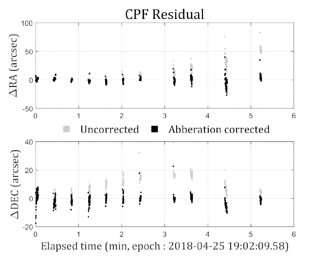
The measurement error models, the light travel time effect and the annual/diurnal aberration, were verified using the OWL-Net data that shall be introduced in section 4. We analyzed the OWL-Net measurement residuals computed by the CPF with and without the corrections. The ephemeris contains approximately 145 daily-state vectors (X, Y, and Z positions) of the target, Cryosat-2, and the position error of the ephemeris is several tens of meters (NERC Space Geodesy Facility 2019). Because the velocity is not provided by the CPF, the position vector at the desired time was obtained by interpolation using the Lagrangian method. Table 1 presents the standard deviation (1σ) values of the measurement residuals before and after the correction. After correction, the RA 1σ was reduced from 8–16 to approximately 5–6 arcsec and the DEC 1σ from 4–10 to approximately 2–7 arcsec, which corresponds to the expected quality level of the OWL-Net observation data (Choi et al. 2018). Fig. 4 shows the measurement residuals of the first arc of the observation. The black dots indicate the corrected residuals, whereas the gray dots represent the uncorrected residuals. The uncorrected residuals tend to be biased owing to the aberration, and the residual became zero-mean by correcting the aberration effect. Note that the light travel time effect was 3.4–5.2 ms, the annual aberration was up to 50 arcsec, and the effect of the diurnal aberration was approximately 1/1,000 of the annual aberration.
In order to verify the LS and UT batch filter, artificial optical observation data were created using GMAT, and numerical simulations were performed using cases with various initial orbit errors. In order to realize a virtual LEO satellite, the initial true orbital elements were set to 7,195.0983 km for the semi-major axis (SMA), 1.2780 × 10⁻⁵ for the eccentricity (ECC), 97.5067° for the inclination (INC), 342.7249° for the RA of ascending node (RAAN), 207.9929° for the argument of perigee (AOP), and 286.1304° for the true anomaly (TA). The reference state vector ( = [–4,981.8931, 842.9225, 5,118.8623] km, = [–4.8963, 2.2328, -5.1458] km/s) converted from the orbital elements at the epoch time (18 February 2016, 18:00:00) was propagated for approximately 8 min with printing the position vector of the ground station in Daejeon, designated as the geodetic longitude of 36.3976°, the geodetic latitude of 127.3757°, and the altitude of 139 m. For the propagation, the Runge-Kutta 9th method was used for the numerical integration and four perturbations were considered: (1) Earth gravitational field model (EGM96 70 × 70), (2) atmospheric drag model (Jacchia-Roberts), (3) solar radiation pressure, and (4) lunar/solar gravity (DE421). The atmospheric drag coefficient was set to 2.0, and the solar radiation coefficient was set to 1.0.
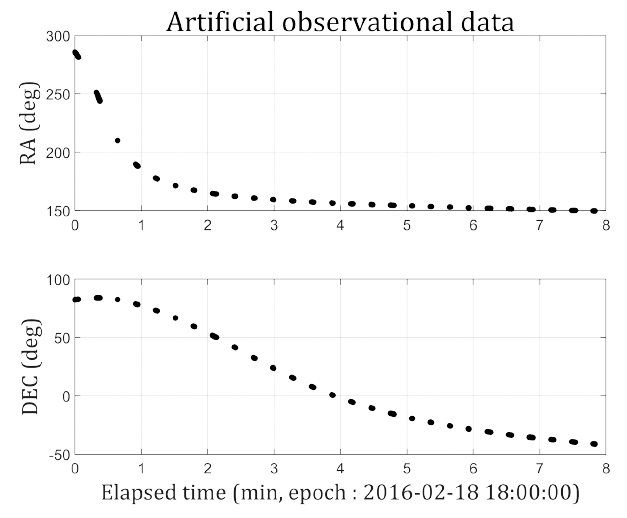
Using the propagated trajectory, the artificial optical observation data composed of topocentric RA and DEC were generated. The optical observation environment was set at 10 Hz for the observation data frequency, 4 seconds for the camera exposure time, 16 seconds for the observational time interval, and 10° for the cutoff angle. Because optical observations can only be performed at night without sunlight, the altitude of the sun was also considered by calculating the solar ephemeris and the observation data were printed only if the solar altitude was less than –10°. Fig. 5 shows the generated virtual optical observational data. RA distributes from approximately 285° to 150° and DEC is spread from approximately 80° to –40°. The total arc length of the observational data is approximately 8 min, and it consists of 570 points of data, extracted from 27 pictures.
POD simulations were conducted using the artificial optical observation data, setting the weight for the observation data as 3 arcsec in both the RA/DEC, and the convergence criterion as 10–3. To include the systematic uncertainty in the simulation, a dynamic model for POD simulation was set as one different to that used for generating the observation data: the JGM3 10 × 10 model for Earth gravitational field; the exponential model for atmospheric density, the analytical approximation for lunar/solar gravity, and the Runge-Kutta 5th method for the numerical integrator.
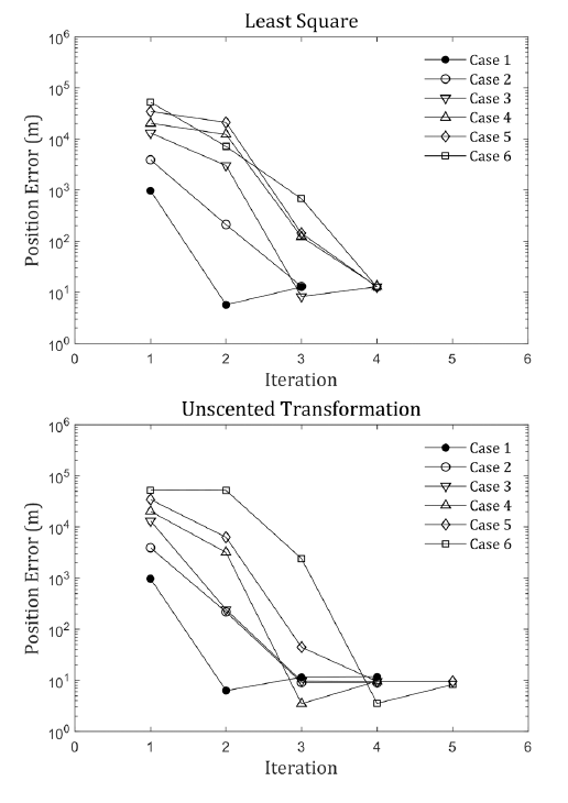
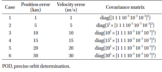
Various initial errors were employed for the simulations, and the effect of the initial error on the accuracy of POD was analyzed. Table 2 shows the initial position/velocity error and the initial covariance matrix of the six cases, and Fig. 6 shows the result of POD according to the initial orbit error. It shows three-dimensional position error at the epoch time with respect to the artificial ephemeris for each iteration, which changes as the iterative computation. Table 3 and Table 4 show the estimated position error between the POD results of LS/UT batch filter and the true ephemeris in the topocentric RTN (radial, transverse, and normal) coordinate system. R is the line of sight of the satellite as viewed from the ground station, T is the direction perpendicular to the R direction in the orbital plane, and N is the direction perpendicular to the orbital plane.
|

|

|
In all the cases, both filters converged within five iterations, and the estimation error from the true ephemeris was approximately 10 m. The artificial LEO satellite orbits a nearly circular orbit with an altitude of 817 km, and therefore, a Gaussian observational noise of 3 arcsec corresponds to a distance error of approximately 12 m on the sky. Therefore, both estimation algorithms converge to the error value corresponding to the observation data quality, and as the optical observation cannot acquire the three-dimensional distance information of the satellite, the position error of the POD result is concentrated in the radial direction. Further, the position error of the UT batch filter is 1–4 m (8%–33%) lower than the error of the LS batch filter in all the cases, thereby indicating improved performance because the UT batch filter is more robust to nonlinear systems than the LS batch filter.
4. OWL-NET DATA APPLICATION
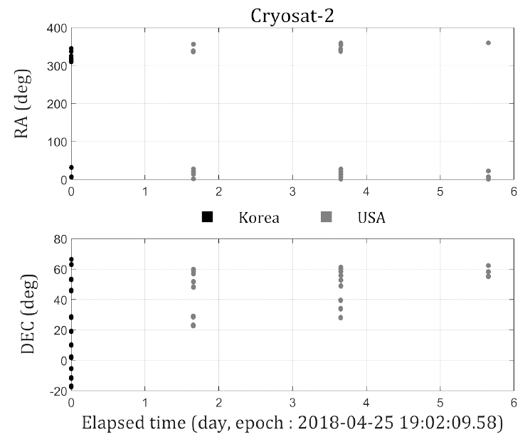
In this section, the real optical observations of Cryosat-2, which has a SMA of approximately 7,096 km and an inclination of approximately 92°, was used, and the corresponding results were analyzed. The data were provided by OWL-Net in April-May 2018 and composed of four arcs where arc 1 was observed in Mt. Bohyun in Korea and arcs 2–4 in Mt. Lemmon in the United States (Table 5; Fig. 7).

|
In the following subsections, the effects of initial error, initial covariance matrix, arc length, and the number of data on POD accuracy have been analyzed. POD accuracy was evaluated by comparing the results to the CPF ephemeris, and the post-fit residuals indicate the RMS error between the observations calculated after the estimation is complete and the real observations corrected with the measurement error model discussed in section 3.1. As in section 3, four perturbation models were considered: (1) Earth gravitational field (JGM3 10 × 10), (2) atmospheric drag (exponential model), (3) solar radiation pressure, and (4) lunar/solar gravity (analytical approximation). There is room for improvement in the accuracy of POD by developing a more precise model later, but in this study, we compared the results by setting the same model for LS and UT batch filters. Note that the atmospheric drag coefficient was set as 1.9 (Choi et al. 2018), and the solar radiation pressure coefficient was set as 0.7 (Root 2012) for the POD. The variance ratios and scaling parameter values used in the estimation are listed in Table 6. β was set as 2, which is an optimal value for the Gaussian distribution (Park et al. 2010), and α was set as 10–3 because the change in α did not significantly affect the POD results in this study. The epoch time of the POD was set as the first observation time, 19:52:19, on April 25, 2018.
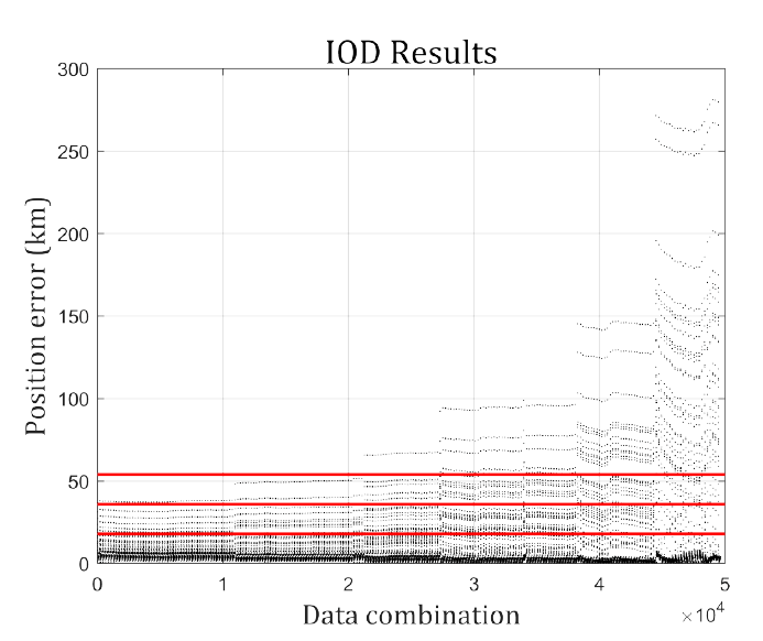
To analyze the effect of the initial orbit error on the POD, various initial error levels were designated. In this study, several initial orbit determination (IOD) results and propagated two-line element (TLE) were employed as initial guessed state vectors to verify that the POD can be performed independently. Gauss’s technique was employed for IOD, which requires three pairs of observational data, , and determines the state vector, , at the intermediate point. The first arc of the observational data consists of a total of 447 data points that were used for IOD, and there were various combinations of observational data: the 232nd data point was fixed as the intermediate point, , and the first point, , and the last point, , were selected from the remaining data. Each IOD result was propagated to the epoch time through the GMAT, and the three-dimensional position error was computed by comparing to the CPF ephemeris, where Fig. 8 shows an error of up to 700 km with a 1σ value of 40.2464 km. To analyze the effect of the initial orbit error on the POD, three combinations were selected from approximately 50,000 combinations and used as the initial guess state vector of the POD. Table 7 lists the position error of the selected initial guesses with respect to CPF in the topocentric RTN coordinates. The position errors of cases 1–3 are concentrated in the radial direction of the ground station because the optical observations cannot acquire the 3D distance information of the satellite. In case 4, however, the concentration is not apparent because the propagated TLE was used as the initial state vector. The initial covariance matrix was set as Pinitial = diag([1 km, 1 km, 1 km, 10–3 km/s, 10–3 km/s, 10–3 km/s]2).

|
Table 8 shows the RMS of the post-fit residuals of POD, and Figs. 9 and 10 show the post-fit residuals of case 1 and case 4, respectively, where the gray dots represent the post-fit residuals of the LS batch filter, and the black dots represent those of the UT batch filter. In cases 2–4, the post-fit residuals converged to several arcsec at both the LS and UT batch filters. However, in case 1, where the initial position error is more than 100 km, the LS batch filter converged to the level of several tens of arcsec. In other words, the UT batch filter converged to the residual level corresponding to the data quality, irrespective of the initial orbit error level, but the LS batch filter exhibited degraded OD performance when the initial orbit error was very large. However, in case 4 which used TLE information, the results of both LS and UT batch filters were similar and the standard deviation value was small.
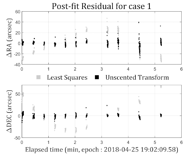
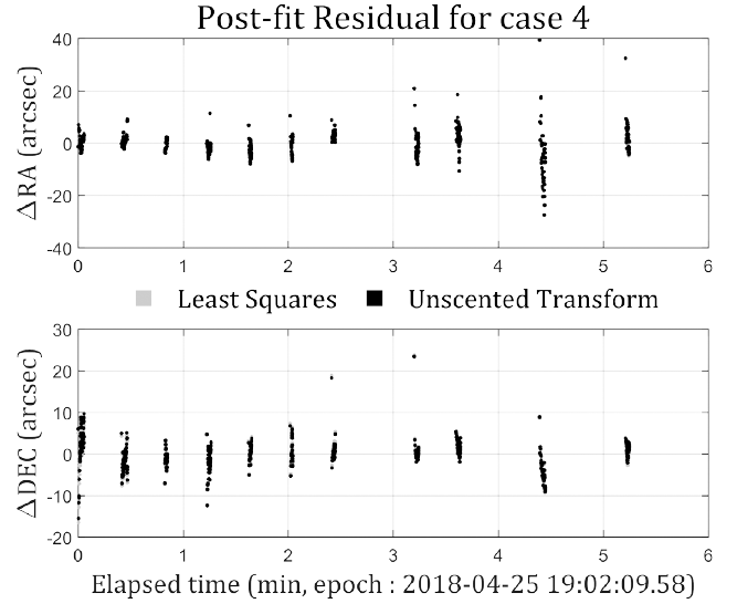
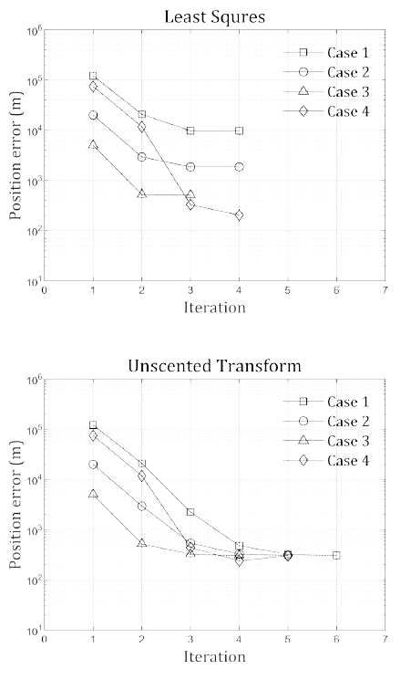
Fig. 11 shows the estimated position error relative to the CPF ephemeris for each iteration, and Tables 9 and 10 show the topocentric RTN position error of the LS and the UT batch filter, respectively. The UT batch filter converged to approximately 300 m in all cases, regardless of the initial error. However, the LS batch filter only converged to the error of several tens of meters in case 3 which had small position error and in case 4 which used TLE information, while it converged to errors of several hundreds of meters in cases 1–2.

|

|
In case 2, the estimated position error was approximately 1,860 m, which is more than three times larger than cases 3–4 results even though the initial position error is 20 km, smaller than that of case 4, and the post-fit residual converged to several arcsec. It might be caused by initial velocity error which is not evaluated by comparing to the CPF data, and the initial guesses were compared to the TLE for analyzing the velocity error indirectly. Tables 11 and 12 exhibit the initial error with respect to TLE. In case 3, the three-dimensional position and velocity errors were 74 km and 78 m/s, which is an order of 1,000 times. In case 1 and case 2, however, the position errors were approximately 120 km and 71 km, while the velocity errors were 605 m/s and 169 m/s, where the velocity error is 2 to 5 times larger than 1/1,000 of the position error. In summary, the initial guesses of cases 1–2 have large velocity error relative to the position error. It can also be concluded that UT batch filter robustly converged regardless of initial velocity error, whereas the LS batch filter is sensitive to the initial velocity error, converging to the local minimum value.

|

|
In order to analyze the influence of the initial covariance matrix on the POD, the initial covariance was variously set while the propagated mean of all IOD results was used as an initial value. The initial position error in the topocentric RTN coordinate system is [14.9560, 3.8612, 0.1869] km, where the error is concentrated in the radial direction of the ground station. The size of the initial covariance matrix is diag (0.32 × [1 km, 1 km, 1 km, 10–3 km/s, 10–3 km/s, 10–3 km/ s]2) for case 1, diag (0.52 × [1 km, 1 km, 1 km, 10–3 km/s, 10–3 km/s, 10–3 km/s]2) for case 2, diag (12 × [1 km, 1 km, 1 km, 10–3 km/s, 10–3 km/s, 10–3 km/s]2) for case 3, diag (22 × [1 km, 1 km, 1 km, 10–3 km/s, 10–3 km/s, 10–3 km/s]2) for case 4, and diag (32 × [1 km, 1 km, 1 km, 10–3 km/s, 10–3 km/s, 10–3 km/s]2) for case 5.
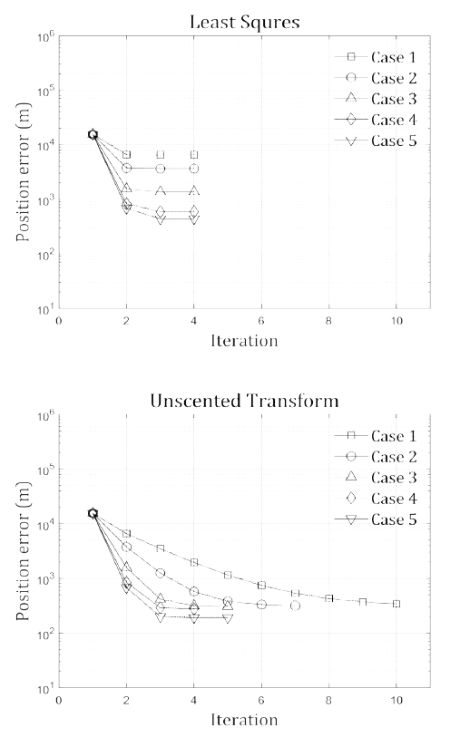
Table 13 shows the RMS of the post-fit residual. In cases 4–5, i.e., with large covariance, both LS and UT batch filters converged similarly to 5 arcsec level in RA and 3 arcsec level in DEC. In cases 1–3, however, the smaller the initial covariance matrix size, the greater the post-fit residual, up to several tens of arcsec in the LS batch filter. In other words, the UT batch filter converged to the residual level corresponding to the data quality in all cases, irrespective of the initial covariance matrix size, but the LS batch filter exhibited degraded OD performance when the initial covariance matrix was small. The initial covariance matrix implies the uncertainty of the initial state vector. When the initial covariance matrix is smaller than the error level of the initial state vector, the LS batch filter converged to the wrong states.

|
Fig. 12 shows the position errors of POD relative to CPF for each iteration, where the upper and bottom are the LS and UT results, respectively. In the case of LS batch filter, the estimation error was several hundred meters in cases 4–5, whereas the position error increased from 1 km to 6 km in cases 1–3. Conversely, the UT batch filter converged to several hundreds of meters, although the estimation error slightly differs for each case. It can be concluded that reliable performance is only achievable for the LS only if the initial covariance is properly designated, but the UT converges robustly regardless of the initial covariance matrix.
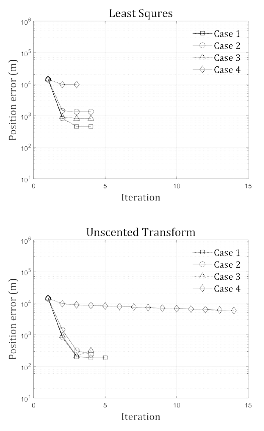
In this section, arcs 1–4 of the OWL-Net data were used to analyze the effects of observation arc length and the number of data points on POD. The arc length is the time between the first data point and the last data point of each arc, which means a single observation image.
The initial guess state vectors were determined in the same way as above: fixing the middle point as the 232nd point for arc 1, the 141st point for arc 2, the 171st point for arc 3, and the 103rd point for arc 4, and choosing the combinations for the Gauss method. Table 14 shows the position error relative to the CPF of the initial guess state vector in the topocentric RTN coordinate system. The initial guesses were selected to contain initial position error of 14.3 km, and the initial covariance matrix is set as Pinitial = diag (32 [1 km,1 km,1 km,10–3 km/s, 10–3 km/s, 10–3 km/s]2).

|
Table 15 shows the RMS of the post-fit residual of the POD. After estimating the precise orbits of all the arcs, the residual converged to the level of 4–6 arcsec in RA, and 2–4 arcsec in DEC, corresponding to the data quality. Fig. 13 shows the POD result as a position error relative to the CPF for each iteration, where the upper shows the LS results and the bottom shows the UT results. Although the measurement residuals converged in all cases, the estimated position vectors did not. For UT batch filter, the estimated position error converged to several hundreds of meters in the case of arcs 1–3. For LS batch filter, the estimated position error was several hundreds of meters in the case of arcs 1 and 3 where the number of observational data points is more than 440. However, in arc 2, where the number of data points is less than 400, the error converged to approximately 1 km level. As the length of arc 2 is approximately 20 seconds longer than arc 3, but the number of data are approximately 50 fewer, the LS batch filter can be analyzed to be more sensitive to the number of data points in the arc than the arc length. The length of the arc 4, meanwhile, is very short, about 60 seconds, and the number of data points is 157. In that arc, both LS and UT batch filter did not converge, and the estimated position errors were 10 km and 6 km, respectively. In conclusion, the POD result could not converge with LS or UT batch filter if more than 400 points of data cannot be obtained for more than 3 min.

|
5. CONCLUSIONS
In this study, POD software for optical observation was developed, verified, and validated by numerical simulations and applying the real satellite observations. For the estimation algorithm, we used batch filter based on the UT to improve the performance over LS batch filter. As a result of the simulation analysis, both batch filters converged to the error level corresponding to the quality of the observed data, regardless of the initial orbit error. At the initial orbit error of under several tens of kilometers, the estimated position error of the LS batch filter was approximately 13 m, whereas the error of the UT batch filter was approximately 8–12 m, which is approximately 8%–33% improved performance.
We also used the real optical observation data of the LEO satellite, Cryosat-2, observed from OWL-Net observatory in April-May 2018. As a result of correcting the effect of light travel time and annual/diurnal aberration using the error model, the standard deviation of measurement residuals with respect to CPF ephemeris was decreased from 8–16 arcsec to 5–6 arcsec for RA, and from 4–10 arcsec to 2–7 arcsec level for DEC. IOD was performed using all data to use as the initial guess state vector for POD. According to the results, the position errors with respect to CPF were at least several tens of meters to several hundreds of kilometers. As a result of the POD for the analysis of the influence of the initial orbit error and the initial covariance matrix, the UT batch filter resulted in post-fit residuals of several arcsec and estimated position errors of several hundreds of meters. However, when the initial orbit error is large or the initial covariance matrix is smaller than initial orbit error level, the LS batch filter failed to converge to the solution, resulting in the residuals of several tens of arcsec and estimation error of several km.
As a result of simulation analysis with various error terms such as initial orbit error and initial covariance matrix, when about 400 observation data were obtained for 3 min or longer, the UT batch filter converged robustly. Furthermore, UT showed improved performance up to 9 km (about 96%) compared to the LS batch filter. In addition, IOD technique was applied to the real optical observations, then the IOD result was used as the initial guess state vector of the POD. In the case of the UT batch filter, the robust convergence was obtained irrespective of the error level of the IOD results. The estimated position error level was similar to TLE. Therefore, it is expected that accurate orbit estimation can be achieved by using IOD and POD software when observational data of a space object or an unknown object, which is not provided with an ephemeris, is secured for a sufficient time. In addition, software performance can be further improved by estimating satellite parameters such as the atmospheric drag coefficient and the solar radiation pressure coefficient.


