Seasonal and local time variations of sporadic E layer over South Korea

1. INTRODUCTION

Sporadic E(Es) represents a thin layer of enhanced electron density in the ionospheric E region. The electron density at Es is 2 – 3 times greater than that of surrounding and even reaches to 10^-12 m^-3. The Es layer has a thickness of about 1 – 2 km and its horizontal length is tens to hundreds of km (Maeda & Heki 2014). In mid-latitudes, the Es layer is formed when the long-lived metallic ions ablated from meteors are converged by horizontal neutral wind shear (Chu et al. 2014;Yeh et al. 2014). The thin Es layer affects radio propagation, and thus hampers to monitor the ionosphere from ground-based GNSS receivers (Hong et al. 2017).

In mid-latitudes, the occurrence rate and intensity (peak frequency, foEs) of Es layers display the typical seasonal variations; they are maximal in summer (e.g. Kelley, 2019 and references therein). This phenomenon is explained by the maximal influx of meteors in summer (Haldoupis et al., 2007). However, it cannot explain why the occurrence rate is not increasing during the Geminids (a meteor shower from Gemini constellation) in the northern hemispheric winter, even though the meteor influx increases during this period. It may be because metallic ions diverge in the E region by the horizontal neutral wind in the ionospheric E region during this period (Yeh et al. 2014). The convergence of metallic ions by wind shear leads to the high occurrence rate of Es in summer, whereas the Es layer is difficult to be formed in winter in spite of abundant metallic ions because of the divergence of horizontal neutral winds. The wind shear also causes the local time variation of Es height as well as the seasonal variations of the Es intensity and occurrence rate. The semidiurnal variation of the Es height in all seasons in midlatitudes is attributed to the semidiurnal variation of the wind shear driven by atmospheric tides (Chu et al. 2014;Oikonomou et al. 2014).

Moreover, the occurrence and intensity of Es is also known to be affected by an intermediate descending layer (IDL), diurnal or terdiurnal tides (e.g. Haldoupis et al. 2006;Oikonomou et al. 2014), non-migrating tide (Sinagawa et al. 2017), lightning (Yu et al. 2015), spread F (Haldoupis et al. 2003;Lee & Chen 2018), and nighttime medium-scale traveling ionospheric disturbances (Otsuka et al. 2008;Ogawa et al. 2009). The intermediate descending layer is a layer between F1 and E layers which occurs irregularly (Haldoupis, 2012). These additional sources of the Es generation complicate the seasonal and local time variations of measured Es parameters.

According to Zhang et al. (2015), in the mid-latitudes, the correlation coefficient between the solar activity and the Es intensity is positive and negative during day and night time, respectively. Moreover, they noted that the electron density of the Es layer increases after the geomagnetic disturbance. Zhou et al. (2017) also reported that the critical frequency of sporadic E (foEs) tends to be larger during the high geomagnetic activity. However, there are also several studies suggesting that the solar and geomagnetic activities do not affect the Es occurrence (Tan et al. 1985;Pietrella et al. 2014). Thus, the Es occurrence and its temporal variation are still not understood in detail, and there may be local effects to be identified.

Despite continuing ionosonde operation in Korea since 1960’s, there has been no study on the Es layer using the Korean ionosonde data. Although it is expected that the Es layer over Korean peninsula follows typical mid-latitude characteristics, it is needed to confirm or disconfirm the characteristics at a quantitative level by using the locally measured data. In this paper, we report the first analysis results of Es layer data measured by ionosondes at Icheon and Jehu. Our analysis focuses on the season and local time variations of Es occurrence and intensity. In addition, to discuss the relation between the vertical ion drift convergence and Es layer height, we compared measured heights of Es layer with the vertical ion drift velocity profiles driven by the horizontal neutral wind which was calculated from the Horizontal Wind Model (HWM) 14 International Geomagnetic Reference Field (IGRF12), and Naval Research Laboratory Mass Spectrometer and Incoherent Scatter Radar (NRLMSISE)-00 model.

2. DATA

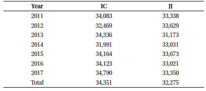
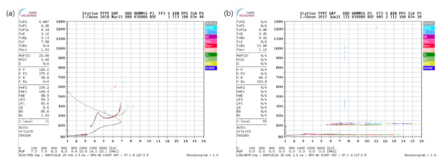
Ionosondes measure the critical frequencies of ionized layers in ionosphere and their virtual heights routinely day and night. The sporadic E data used in this study were obtained from the ionosonde measurements at Icheon (37.14°N, 127.54°E, IC) and Jeju (33.4°N, 126.30°E, JJ) in 2011 – 2018. The ionosondes carry out the vertical incidence observation with a time interval of 15 min as well as the oblique incidence observation between Korea and Japan. We used only vertical incidence data. Table 1 shows the number of available ionograms at IC and JJ. Fig. 1(a) and 1(b) show typical ionograms without and with a sporadic E layer, respectively, measured at IC. The sporadic E layer clearly appears as a thin layer of echo signals at the bottom of Fig. 1(b). To investigate the occurrence rate of the Es layer, we calculated the Es occurrence rate as follows:

Table 1. The number of available ionograms measured by the Icheon (IC) and Jeju (JJ) ionosondes during a period of 2011 – 2018.

Download Excel Table

Fig. 1. a) An example of a normal ionogram (no sporadic E layer), b) an ionogram with a sporadic E layer measured at Icheon station.

Download Original Figure

The IC and JJ ionosondes are a type of the digisonde, Digisonde Portable Sounder 4D (DPS4D). The observations of the ionosondes are analyzed by a software of Automatic Real-Time Ionogram Scaling with True analysis (ARTIST-5) and then saved as a format of Standard Archiving Output (SAO). The auto-scaled data can be downloaded at the website of the Korean Space Weather Center (http://spaceweather.rra.go.kr/). Although the Jeju auto-scaled F2 parameters were evaluated to differ by 36% from manually scaled ones (Jeong et al., 2018), the auto-scaled Es parameters are expected to be more accurate than the auto-scaled F2 parameters since the Es layer is significantly easy to be defined automatically.

3. RESULTS AND DISCUSSION

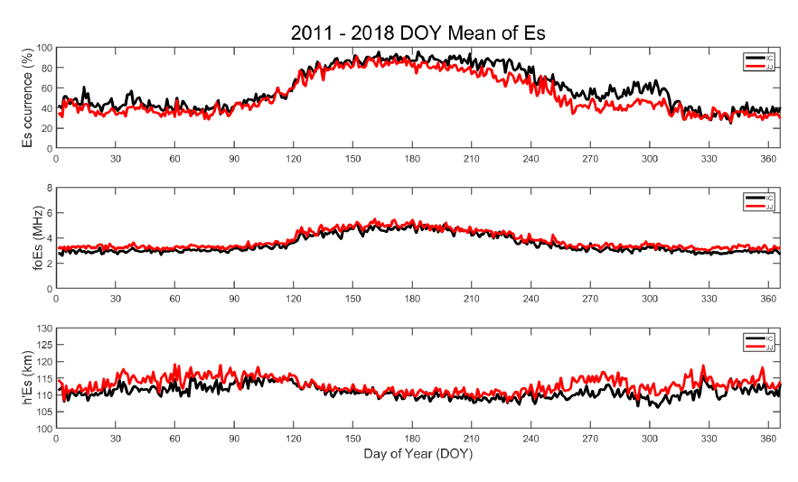
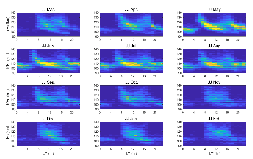
Fig. 2 displays the seasonal variations of the Es occurrence rate at IC (black line) and JJ (red line). The occurrence rate on each day is obtained using the data in 2011 - 2018. In Figs. 2(a) and 2(b), the Es occurrence rate and the magnitude of foEs have the peak values in summer season in consistent with their known seasonal pattern in midlatitudes (Haldoupis, 2012). This behavior is related to the wind shear and meteor influx in summer (Haldoupis et al. 2007;Arras et al. 2008;Chu et al. 2014;Yeh et al. 2014). However, the virtual height of Es (h’Es) shows the semiannual variation at both IC and JJ with two peaks in equinoxes (Figure 2c). Meteor radar measurements have reported that peak altitudes of meteors vary in a similar manner around the mesopause altitude (Lee et al. 2016). The meteor peak variation is interpreted as a consequence of seasonal geopotential height change. The seasonal variation of h’Es may be related to the meteor peak height variation since the atmospheric change around the mesopause will affect the background atmosphere at the Es layer. Further investigation is needed to test the relation between variation of h’Es and meteor peak heights.

Fig. 2. Seasonal variations of the Es observed during the year of 2011 – 2018 at Icheon (black line) and Jeju (red line). The X-axis and Y-axis are the day of year and the occurrence rate, respectively.

Download Original Figure

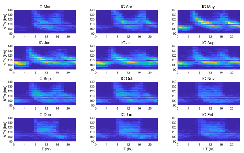
Maps of Es occurrence rate as a function of time and height at IC and JJ are shown in Figs. 3 and 4, respectively. The time and height bins of the plot are 1 hour and 1 km. In both IC and JJ, h’Es shows a semi-diurnal variation that has two distinct peaks at early morning and the other at late afternoon. The semi-diurnal variation is most pronounced in summer, but the two peaks are not obvious in winter. Similar phenomena were identified at different regions (e.g. Oikonomou et al. 2014;Chu et al. 2014).

Fig. 3. Monthly height-time-occurrence rate of Es at Icheon.

Download Original Figure

Fig. 4. Monthly height-time-occurrence rate of Es at Jeju.

Download Original Figure

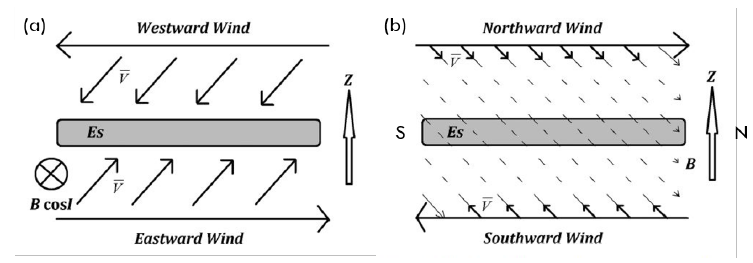
Theoretical studies have proposed a scenario that the Es layer is formed when the metallic ions are converged by the neutral wind shear in the mid-latitudes (e.g. Chu et al. 2014). Fig. 5(a) illustrates the Es layer formation by the zonal wind shear. When the eastward zonal wind blows, the ions are vertically upward drifted by $\overrightarrow{U}\times \overrightarrow{B}$ where $\overrightarrow{U}$ is zonal wind velocity and $\overrightarrow{B}$ is geomagnetic field. In contrast, the westward zonal wind drifts the ions downward. In addition, the ion-neutral collision is frequent in the ionospheric E region because of the high atmospheric density, so that the meridional wind can move the ions along the geomagnetic field line. For example, in the northern hemispheric mid-latitudes, the meridional wind moves the ions as shown in Fig. 5(b), thus the Es layer forms by the ion convergence (Chen et al. 2010;Yeh et al. 2014;Haldoupis, 2012). In the geomagnetic equatorial region, the geomagnetic field lines are almost parallel to the horizontal, so that the meridional wind can only move ions easily along the lines. On the other hand, the zonal wind can move ions vertically by $\overrightarrow{U}$×$\overrightarrow{B}$. However, the zonal wind cannot easily form the Es layer because ions are fixed to the geomagnetic field lines in the E-region altitudes, where the ion- neutral collisional frequency is much greater than the ion gyro-frequency. In the high-latitudes, the horizontal component of the geomagnetic field lines is too small to form the Es layer by zonal and meridional wind. Therefore, the Es formation by wind shear is difficult in the geomagnetic equatorial and high-latitude regions.

Fig. 5. Illustration of the wind shear convergence mechanism for ions in the northern hemisphere (Yeh et al. 2014). (a) The E_S layer formation by the zonal wind shear. (b) The Es layer forms by the meridional wind shear.

Download Original Figure

Following the formula in Mathews (1998), the vertical ion drift velocity (w) can be expressed as a function of the zonal and meridional wind velocities,

where U and V are the zonal and meridional wind velocities, respectively. Note that eastward zonal wind velocity is set to be positive, and I is the dip angle calculated from the International Geomagnetic Reference Field (IGRF). ν_i/ω_i is the ratio of the ion-neutral collision frequency to the ion gyro-frequency, which can be calculated by the Eqs. (3) and (4) (Yuan et al. 2014).

where m₊ is the average ion mass, e and B₀ are electron charge and magnetic field, A is the metallic ion mass, $n_{N_2},\hspace{0.33em}{n}_{O_2},\hspace{0.33em}\text{and}\hspace{0.17em}{n}_O$ are the number densities of the N₂, O₂, and O, respectively. The meridional wind term can be neglected in the Eq. (2) because of ν_i≫ω_i below the altitude of 120 km. Thus the vertical ion drift velocity is mainly controlled by the zonal wind term in the ionospheric E region.

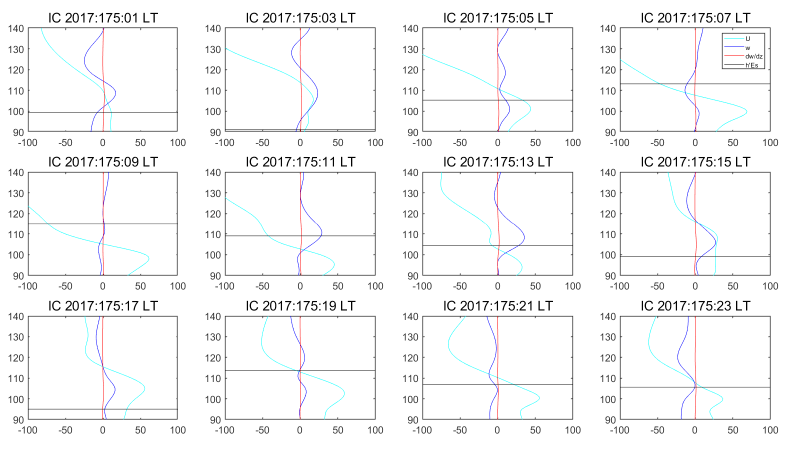
In this study, we investigated the correlation between the gradient of the vertical ion drift velocity with the altitude dw/dz and the h’Es. To compute the vertical ion drift velocity profile, we adopted neutral densities from the NRLMSISE-00, and the neutral winds from the Horizontal Wind Model (HWM14). When the eastward and westward winds are blowing at low and high altitudes, respectively, as shown in Fig. 5(a) the dw/dz is negative. That is, the dw/dz < 0 represents the ion convergence, whereas the dw/dz > 0 means the ion divergence.

Fig. 6 shows the profiles of the zonal wind velocity (U), vertical ion drift velocity (w), and dw/dz, which are calculated from 90 to 140 km, and the 1 hour mean h’Es at IC on the day of June 24, 2017. The cyan, blue, red, and black lines are the U, w, dw/dz, and h’Es, respectively. The Es layers appear under the altitude of 100 km from midnight until dawn (01 – 04 LT), which may not be related to the vertical ion drift because the ionospheric E region normally disappears at nighttime due to fast recombination of molecular ions produced during daytime. The E_S layers may be caused by in situ meteor ablation and survive because of slow recombination of metal atomic ions (Fe⁺, Mg⁺, Na⁺) (see Kelley, 2009). After 04 LT, except 14 – 17 LT, the Es layers occur around the altitude where the dw/dz is minimum, that is, the vertical ion convergence is maximum. During 14 – 17 LT, the Es layers tend to form around where the first (lower altitude) minimum of dw/dz. The profiles and h’Es at JJ on the day of June 27, 2017 are displayed in Fig. 7. The local time variations of the profiles and h’Es are similar to the Fig. 6. Therefore, the semidiurnal variation of h’Es is related to the variation of vertical ion drift which was driven by semidiurnal tide of neutral winds. However, the nighttime Es occurrence, especially from midnight to dawn, is not consistent with the vertical ion drift.

Fig. 6. Vertical profiles of the zonal wind velocity (cyan), vertical ion drift velocity (blue), and dw/dz (red) from 90 to 140 km, and h'ES (black) at IC in the day of June 24, 2017. The numbers in x-axis are in units of m/s and 10^-3 s^-1 for wind and drift velocities, and dw/dz, respectively.

Download Original Figure

4. CONCLUSIN AND SUMMARY

We have investigated the occurrence climatology of Es using the measurements of ionosondes at IC and JJ in 2011-2018. In both stations, the occurrence rate of Es and the magnitude of foEs show the maximum values in summer, confirming previous studies of mid-latitude Es (Haldoupis et al. 2007;Chu et al. 2014;Yeh et al. 2014). However, the h’Es shows semi-annual variation with two peaks in equinox months, similar to that of meteor peak heights in the mesosphere measured by a meteor radar at King Sejong Station (Lee et al, 2016). The local time variations of the h’Es shows the semidiurnal modulation during equinox months and summer months, which is consistent with the results in previous studies (e.g. Haldoupis et al. 2006;Oikonomou et al. 2014). However, the semi-diurnal variation is not obvious in winter. Our calculation of the vertical ion velocity using HWM14, IGRF12, and NRLMSISE-00 models support the association of the semidiurnal variation of h’Es with the semidiurnal variation of tidal horizontal wind.