


1 INTRODUCTION
The safe and normal operation of satellites requires the maintenance of sufficient power for attitude control, communication, and other missions. Satellites produce power through solar panels during daylight, some of which is used in each subsystem while the satellite is in operation, and the rest of which is stored in a battery for use when it is impossible to produce power. The power produced by the solar panels must be greater than the power consumed by the satellite. If the generated power is lower than the consumed power, the satellite may stop operating or the life of the satellite may be reduced. On the other hand, if the generated power is excessive, the solar panels may overheat, introducing heat into the system. Therefore, it is critical to produce an appropriate amount of power.
In this study, a power analysis program was developed using MATLABⓇ to verify the power balance inside a satellite during operation. The MATLABⓇ graphic user interface (GUI) was used for user convenience. In South Korea, three continuous orbits were operated in a study for testing the generation of power for each orbit (Lee & Ra 2007). In another study, an energy balance analysis program of a low earth orbit satellite was developed to verify the efficiency of missions and energy balance by predicting the depth of discharge (DOD), bus voltage, and charge/discharge currents (Jeon et al. 2010). In an overseas study, a program for analyzing the solar panel and battery power according to the orbit rotations of a cube satellite Missat-1 was developed (Gordji et al. 2014). However, these previous studies only analyzed the power of low earth orbit satellites, and universal power analyses with ultra-small earth observation satellites for observing multiple points at various angles with satellites were rare. In the present study, a power analysis program was developed for cube satellites with various earth observation missions. As this program was developed for general purposes, it can be applied to various shapes and sizes of satellite models. This program can be used to verify the appropriate power balance inside a satellite in operation and will aid selection of the appropriate power budget during the design of a power system. In addition, this program will help researchers check the energy balance of a satellite in operation and therefore solve problems as they arise.
2 CONFIGURATION OF THE PROGRAM
When designing a power system, a power budget is selected to supply sufficient power to each subsystem and to prevent power consumption from exceeding the available amount of power. This allows researchers to avoid emergencies, such as power shortage, during satellite operation. If the power capacity is designed to be greater than the required power, cost problems and other various problems in the thermal control system, power system, and propulsion system may occur. A large power system cannot be designed for a cube satellite owing to the small size of the satellite body. Therefore, it is crucial to design an appropriate power capacity and maintain power balance for stable satellite operation.
Energy balance analysis (EBA) is carried out to check whether the generated power of the satellite is balanced with the power consumption and the stored power. The magnitude of each power is compared, and the status of power is predicted so that the power produced from the solar panel during daylight, the power consumed in each subsystem, and the power stored in the battery maintain the optimal condition.
The satellite power system designed using the proposed program will allow us not only to design the appropriate power capacity for the power system of a satellite, but also to calculate the power through simulation even while the satellite is operating in an orbit, and determine the possibility of stable operation.
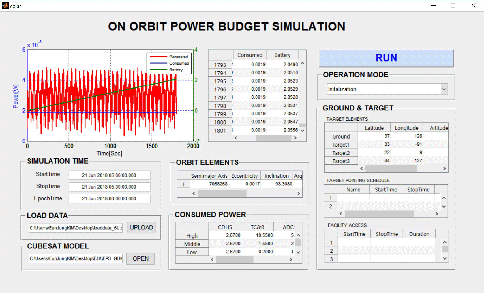
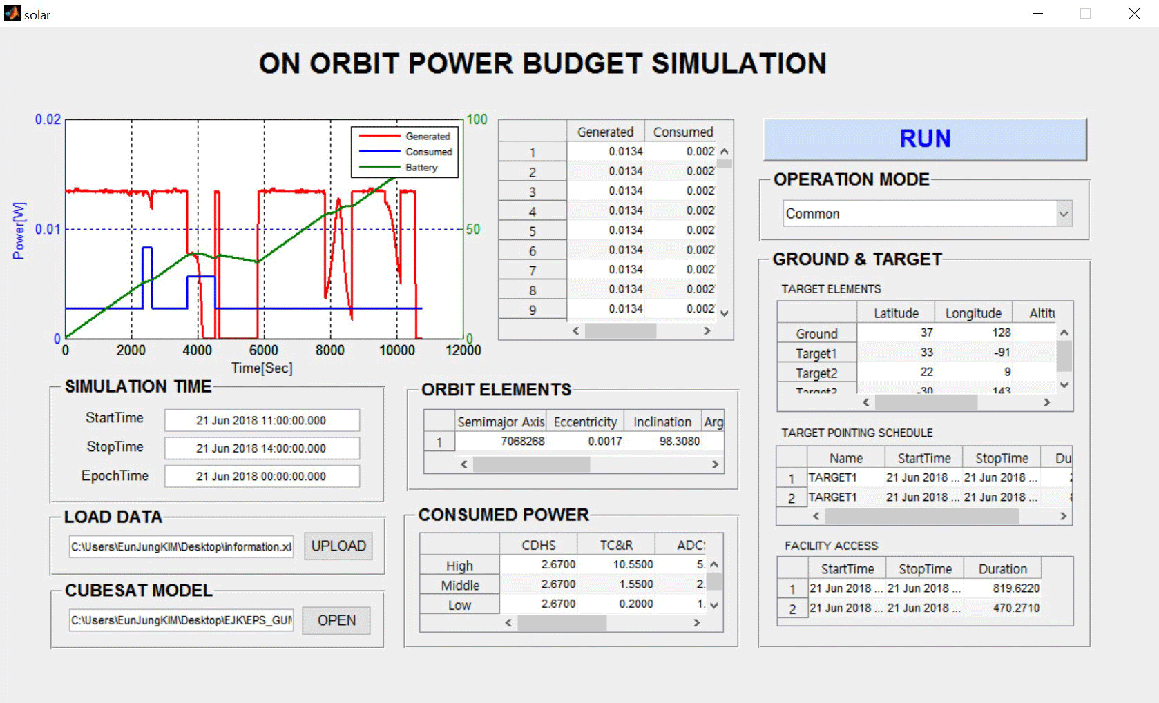
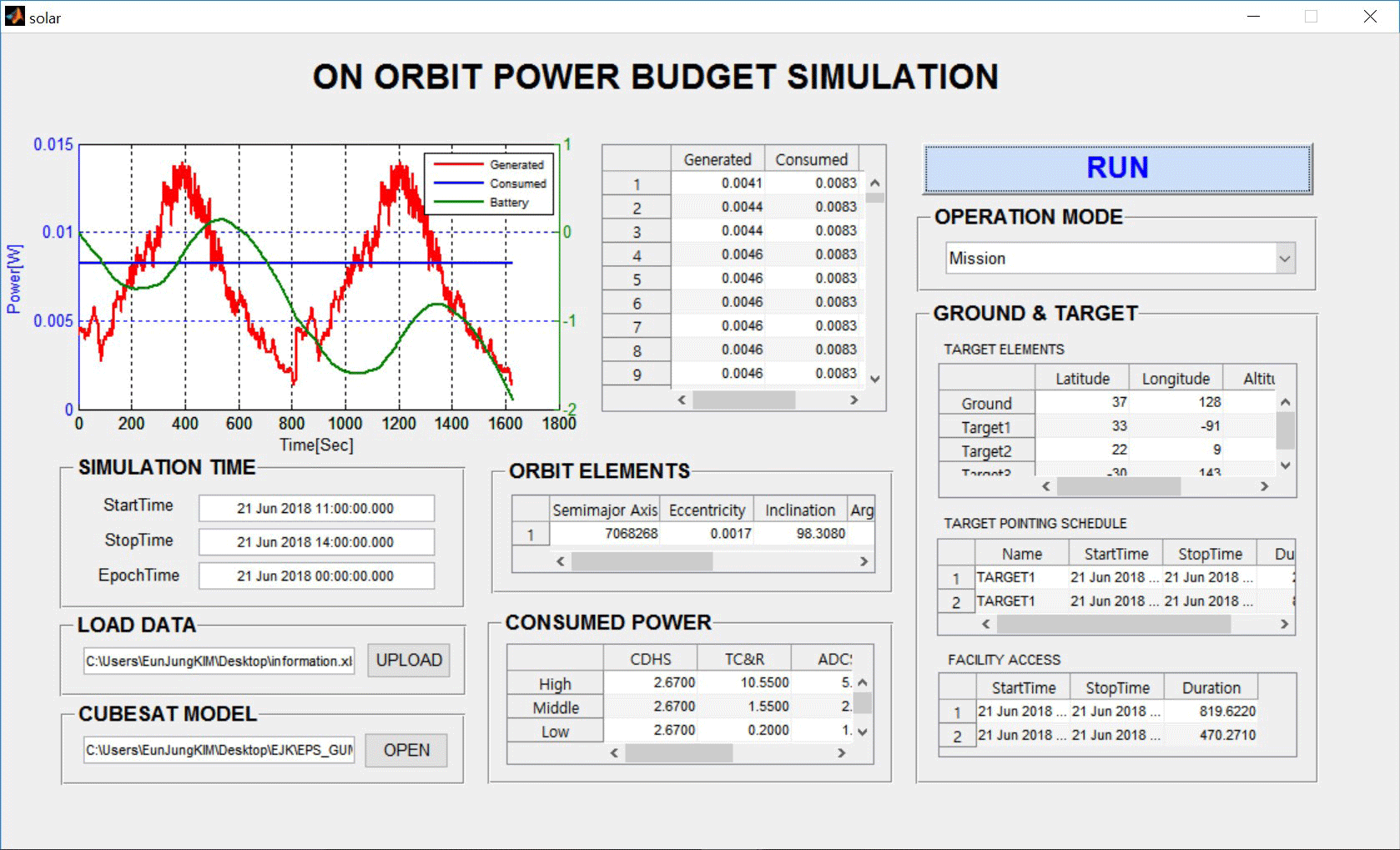
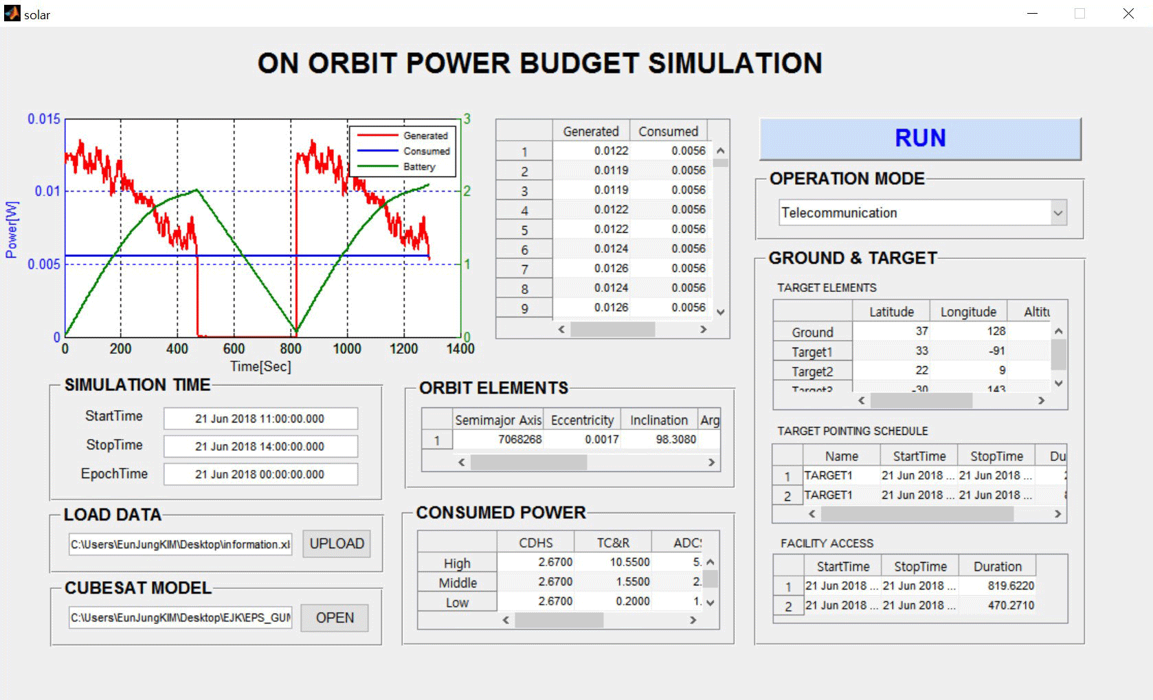
The simulator was produced with MATLABⓇ GUI for user convenience and the input components included simulation time, orbit elements, ground & target elements, consumed power, CubeSat model, and operation mode. When the RUN button at top right was clicked after entering these elements, the simulation started, and the generated power, consumed power, and battery power were calculated. A graph of the analysis results appears in parts ⓐ at the top left in Fig. 1, and the resulting values appear in a table in part ⓑ at the top center.
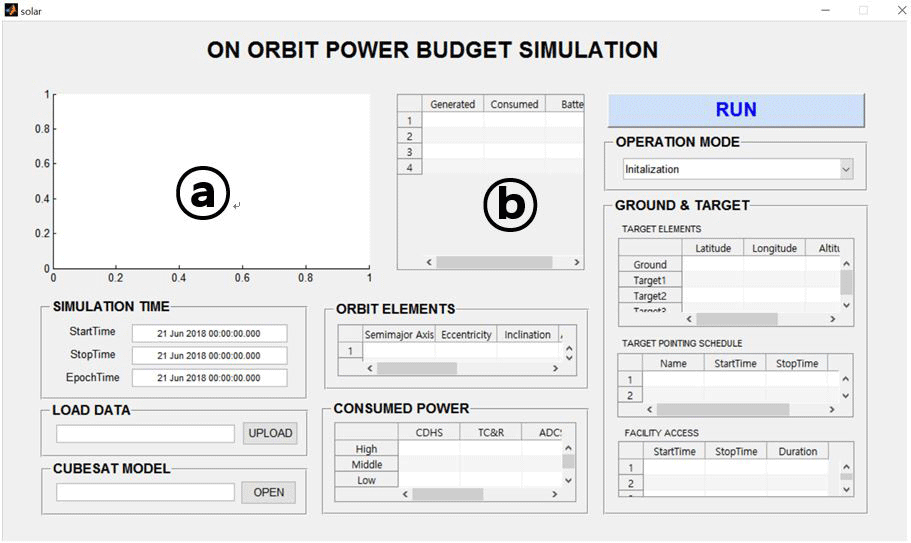
The simulation time was designed so that inputted text could be received directly on the GUI, and as a result, changes over time could be checked frequently during simulation. In the case of orbit elements, ground & target elements, and consumed power, which have a large amount of data and for which the initial settings during simulation change rarely, the values were entered in an Excel document and the Excel file was uploaded to input the data to eliminate the inconvenience. Furthermore, the orbit elements, consumed power, and target elements were listed in tables so that the user could easily see the input values at a glance. To check the communication sections of the satellite, the starting and ending times and time duration were added using the target pointing schedule and facility access tables
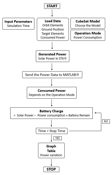
Fig. 2 shows the flow chart of the program. When you enter the parameters and click the RUN button, the generated power of the solar panel is calculated through the solar panel power simulation in STKⓇ, which is linked to MATLABⓇ. The power produced here is instantaneous power, calculated in seconds for precision. Then the calculated values are automatically input into MATLABⓇ, and the battery power is calculated through the generated power and consumed power. The calculation is performed only for the time set on GUI, and the power variation over time is displayed in the graph and tables on the GUI.
The STKⓇ power simulator receives the generated power in instantaneous power (W) units. However, the calculated result is displayed in power (Wh), as shown in Eq. (1), which is the product of instantaneous power (W) and hour (hr).
The power consumption that has been input and the power generated in STKⓇ are both instantaneous power, and should be converted to power (Wh) by Eq. (2) in order to determine the power capacity. The power P(Wh) is an integrated value of the instantaneous power p(W) as well.
Furthermore, remaining battery power is the generated power minus the consumed power in the second unit, and it was assumed that all the remaining power was converted to battery power, as expressed by the following equation:(3)
The simulation time is from t1 to t2.
The major input components are as follows:
-
Simulation time
This consists of start time, stop time, and epoch time, and the time interval is one second.
-
Orbit elements
There are six orbit elements that determine the operated orbit. They include semimajor axis, eccentricity, inclination, argument of perigee, RAAN, and mean anomaly. For the data in Table 1, the orbit elements of the Arirang 2 satellite were referenced (Seong et al. 2013).
-
Ground and target elements
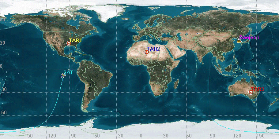
The locations of the ground station and mission target are specified through the latitude, longitude, and altitude. Only one ground station was set because the satellite in this study was a cube satellite, and up to three targets could be set. The location of the ground station presented on Table 2 refers to the Daejeon ground station, and for the location of targets, one target was selected randomly for each continent. The locations of the ground station and targets on 2D graphic are given in Fig. 3.
-
Consumed power
The power was input in high, medium, and low sizes of the instantaneous power for each subsystem. For the data in Table 3, the power budget of a 6U cube satellite for earth observation using an optical camera HiReV (High Resolution Image & Video) was referenced (Kim et al. 2016).
-
CubeSat model
The model of a cube satellite is required for the STKⓇ solar panel simulation for power generation. The model shape varies by the function and capacity of each satellite.
| Semi-major | Eccentricity | Inclination | Perigee | RAAN | M. Anomaly |
|---|---|---|---|---|---|
| 7068268 | 0.001656 | 98.308 | 115.25 | 29.706 | 245.042 |
| Latitude | Longitude | Altitude | |
|---|---|---|---|
| Ground | 37 | 128 | 0 |
| Target1 | 33 | -91 | 0 |
| Target2 | 22 | 9 | 0 |
| Target3 | -30 | 143 | 0 |
| CDHS | TC&R | ADCS | EPS | Payload | |
|---|---|---|---|---|---|
| High | 2.67 | 10.55 | 5.535 | 1.29 | 20.095 |
| Medium | 2.67 | 1.55 | 2.665 | 1.29 | 0 |
| Low | 2.67 | 0.2 | 1.665 | 1.29 | 0 |
The five modes that are most generally used for analysis of cube satellites were selected as the operation modes of this simulator (Kim 2007).
-
Initialization mode
The status of the satellite is checked in the early stage of satellite operation; the antenna is unfolded and the communication and power systems are initialized. The solar panel is not unfolded yet.
-
Common mode
The satellite travels in an orbit with the solar panel unfolded with no mission or communication.
-
Mission mode
The satellite performs its own missions such as capturing images of the specified areas using mounted devices such as optical cameras.
-
Telecommunication mode
The data obtained from the mission is communicated with the ground station.
-
Safe hold mode
When the power supply is insufficient, the satellite is operated with minimum functions and minimum power.
Table 4 shows the power consumption of each subsystem by operation mode. The magnitudes of power of the subsystems are categorized as high, medium, and low.
| CDHS | TC&R | ADCS | EPS | Payload | |
|---|---|---|---|---|---|
| Initialization | H | L | M | H | L |
| Common | H | L | H | H | L |
| Mission | H | L | H | H | H |
| Telecommunication | H | H | H | H | L |
| Safe Hold | H | M | M | H | L |
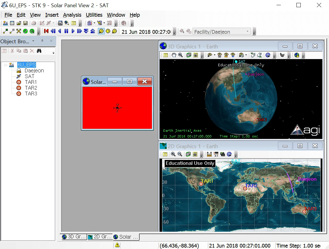
The data of the STKⓇ, such as generated power and com- munication time, were directly sent to MATLABⓇ. When the input elements are inputted in the GUI and the simulation is carried out, the STKⓇ execution screen appears as shown in Fig. 4. The STKⓇ simulation can only check the generated power of the solar panel. The generated power data in the STKⓇ is listed in Table 5.
The different types of power were calculated in five operation modes with a 6U cube satellite and were compared with the results obtained in the common mode. The simulation time intervals were set in seconds. The power changes are shown in Fig. 5. The scale on the x-axis indicates the time (seconds). The red line represents the generated power, the blue line consumed power, and the green line remaining battery power. The left-side scale on the graph represents the size of the generated power and consumed power, and the right-side scale represents the remaining battery power. The initial value of batter power was set to zero to examine the power supply status in the worst situation.
-
Initialization mode
This is the process of checking and initializing the satellite status immediately after the satellite enters the orbit. The simulation time was set to 30 min. Because this mode precedes the unfolding of the antenna and solar panel, the satellite does not perform any missions or communication, such as orientation to the target or ground station. Fig. 5 shows the analysis results. At the beginning of the orbit, the satellite rotates with a tip-off rate to attitude, so the generated power graph has the following fluctuation. Table 6 shows the sizes of generated power, consumed power, and battery power. The consumed power shows the general values excluding missions and communications.
-
Common mode
The simulation time of the common mode was set as 3 hr to observe results for the two cycles. As shown in Fig. 6, two target orientations and ground station orientations were observed. The variations in the power data according to the satellite orientations can be seen. Table 7 shows the power data and the consumed power increased from 0.019 Wh in the initialization mode to 0.027 Wh because the satellite, in this mode, was carrying out a mission. With the start of fullscale operation, the battery power increased from 20.725 Wh to 78.16 Wh.
-
Mission mode
This mode shows only the results in the common mode that were generated during the performance of missions by the satellite. As can be seen in the target pointing schedule under ground and target section in Fig. 7, the satellite aims at the target twice during the simulation, for around 3 hr. These two groups of data appear continuously in the graph. In Table 8, the remaining battery power is –0.041 Wh, which is a negative value. This means that the power supply is insufficient when the initial value of battery power is zero. Furthermore, the generated power decreased from 0.0134 Wh in the common mode to 0.0122 Wh because the satellite could not aim at the sun owing to a change in the attitude of the satellite.
-
Telecommunication mode
The telecommunication mode shows the results in the common mode that were generated while the satellite was aimed at the ground station. Because the satellite aimed at the ground station a minimum of two times, the corresponding graphs appear in succession. The simulation results are shown in Fig. 8 and Table 9. As with the mission mode, the generated power of the solar panel decreased from 0.0134 Wh in the common mode to 0.0122 Wh owing to a change in the attitude of the satellite.
-
Safe hold mode
In this mode, the satellite operates with minimum functions because it has a problem. The result graph is shown in Fig. 9. Thus, as the result shown in Table 10, the satellites can’t aim for the sun. So solar panels couldn’t generate the power at all, but the power consumption still continue, so the remaining battery power becomes negative.
| Max Generated Power (Wh) | Avg Consumed Power (Wh) | Max Battery Power (Wh) |
|---|---|---|
| 0.0056 | 0.019 | 2.0556 |
| Max Generated Power (Wh) | Avg Consumed Power (Wh) | Max Battery Power (Wh) |
|---|---|---|
| 0.0134 | 0.027 | 78.16 |
| Max Generated Power (Wh) | Avg Consumed Power (Wh) | Max Battery Power (Wh) |
|---|---|---|
| 0.0122 | 0.083 | -0.041 |
| Max Generated Power (Wh) | Avg Consumed Power (Wh) | Max Battery Power (Wh) |
|---|---|---|
| 0.0122 | 0.056 | 2.08 |
| Max Generated Power (Wh) | Avg Consumed Power (Wh) | Max Battery Power (Wh) |
|---|---|---|
| 0 | 0.023 | -0.079 |
If the satellite size increases, the number of cells on the solar panel also increases, which in turn increases the generated power per area. As the weight of components increases, the consumed power according to the operation mode also increases. Conversely, if the satellite size decreases, the area of solar panel decreases, which in turn decreases the generated power. Furthermore, as the weight of components decreases, the consumed power also decreases.
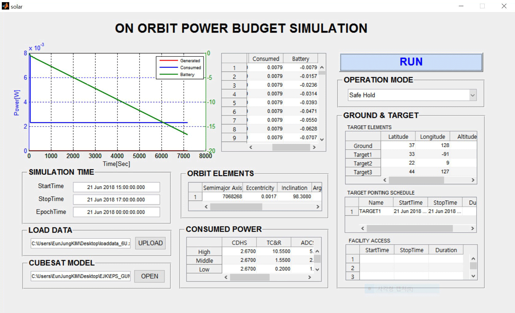
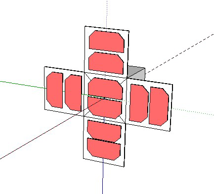
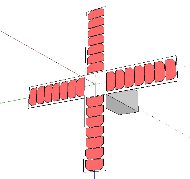
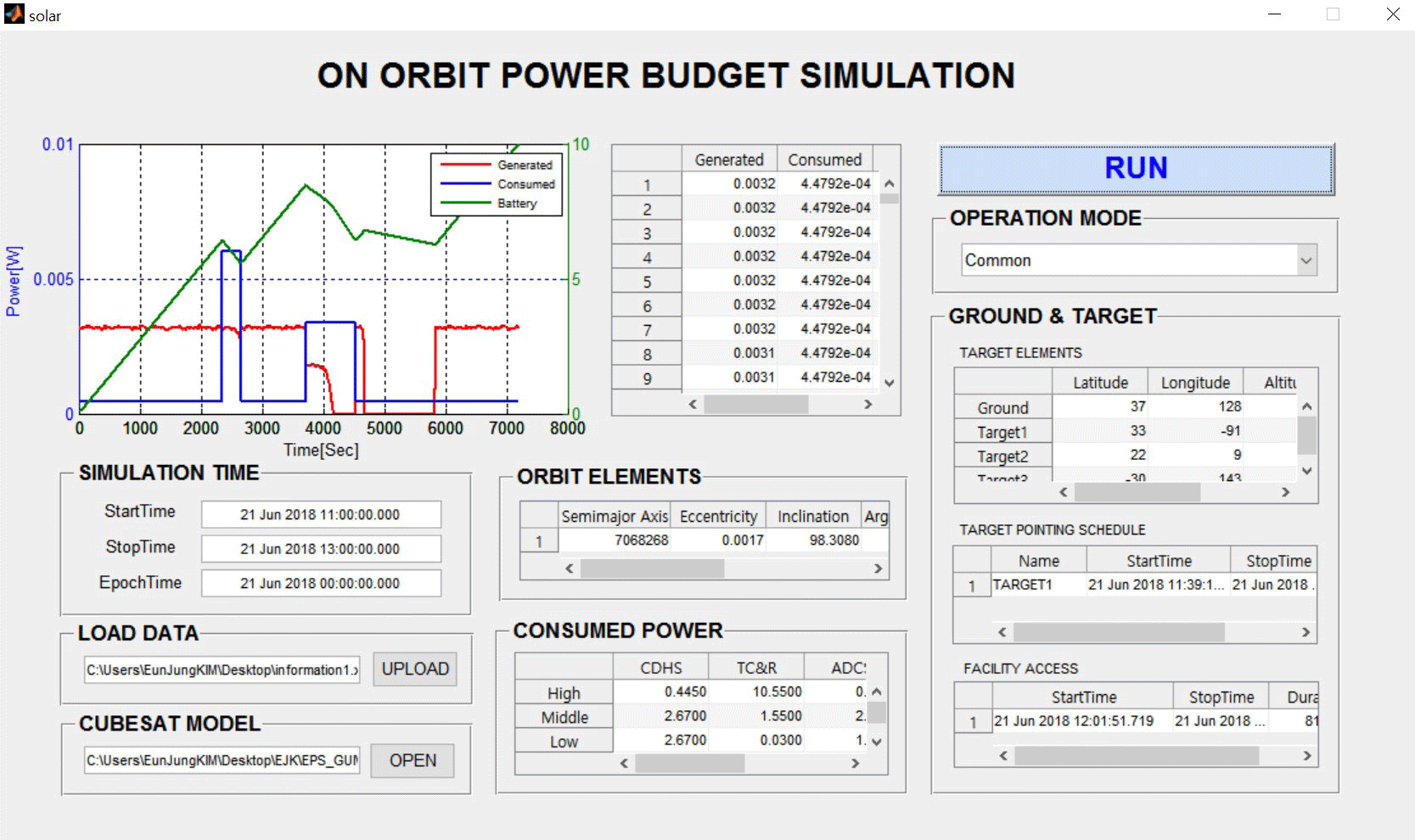
For this simulation, a 1U cube satellite in Fig. 10 and a 3U cube satellite in Fig. 11 were applied, and the analysis results of these satellites in the common mode were compared with the analysis results in the common mode of the existing 6U-class cube satellite. The shape of the 6U cube satellite is shown in Fig. 12.
-
1U CubeSat
In the case of the 1U cube satellite, the area of the solar cell and the consumed power of each subsystem also decreased with a decrease in the capacity and size of the satellite. The consumed power of the 1U satellite is shown in Table 11, and the calculated size of each type of power (Wh) is shown in Fig. 13.
-
3U CubeSat
The consumed power of the 3U cube satellite is shown in Table 12, and the simulation results are shown in Fig. 14. The capacity of the 3U cube satellite was only half of that of the 6U cube satellite, but about three times that of the 1U cube satellite. Thus, the consumed power of each subsystem increased three-fold compared with that of the 1U cube satellite and decreased two-fold compared with that the 6U cube satellite.
| CDHS | TC&R | ADCS | EPS | Payload | |
|---|---|---|---|---|---|
| High | 0.445 | 1.76 | 0.9225 | 0.215 | 3.35 |
| Medium | 0.445 | 0.258 | 0.44 | 0.215 | 0 |
| Low | 0.445 | 0.03 | 0.2775 | 0.215 | 0 |
| CDHS | TC&R | ADCS | EPS | Payload | |
|---|---|---|---|---|---|
| High | 1.335 | 5.28 | 2.77 | 0.645 | 10.05 |
| Medium | 1.335 | 0.774 | 1.32 | 0.645 | 0 |
| Low | 1.335 | 0.09 | 0.8325 | 0.645 | 0 |
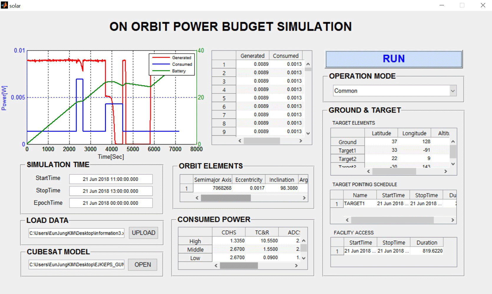
The generated power of each subsystem is related to the number of solar cells, and the number of solar cells in each unit is outlined in Table 13. The number of solar cells of the 1U satellite was smaller by around four fold compared to that of the 6U satellite; furthermore, the number of solar cells of the 3U satellite were 2/3 times that of the 6U satellite.
| Unit | 1U | 3U | 6U |
|---|---|---|---|
| Number of Solar Cell | 10 | 28 | 42 |
The powers of these satellites were compared and the power variations by satellite size are outlined in Table 14. Because the generated power is proportional to the number of solar cells, the generated power of the 1U satellite decreased by four fold compared to that of 6U satellite, and the generated power of the 3U satellite was 2.3 times that of the 6U satellite. The remaining battery power was also proportional to the generated power and consumed power.
| Unit | Max Generated (Wh) | Avg Consumed (Wh) | Max Battery (Wh) |
|---|---|---|---|
| 1U | 0.0032 | 0.0004 | 9.86 |
| 3U | 0.0089 | 0.0013 | 38.05 |
| 6U | 0.0134 | 0.027 | 78.16 |
The power variations according to the operation mode and satellite size were examined to investigate the energy balance and power capacity of each satellite. First, to examine the variation by operation mode, simulations were performed with only the 6U cube satellite in different operation modes. Then, to examine the variations by satellite size, simulations were performed with 1U and 3U cube satellites in common modes for the same duration. The graphs above show that the generated power decreased as the satellite size decreased under the same conditions. In addition, the consumed power and battery power also decreased, which in turn decreased the total power capacity.
The generated power decreases when the satellite cannot aim at the sun during an eclipse or due to a change in the attitude of satellite. The consumed power of the communication system or mounted device increases depending on the orientation toward the ground station or target, thus increasing the values on the graph as well.
3 CONCLUSIONS
In this study, a program for analyzing the energy balance of satellites was developed using MATLABⓇ, and the correct operation of this program was verified through simulations by operation mode and satellite unit. In order to instantly send the power generated in STKⓇ to MATLABⓇ, data processing was accelerated and simplified through the MATLABⓇ-STKⓇ interface. Furthermore, by receiving the input values through file uploading, the input process was simplified.
First, the power variations in five operation modes were verified with the 6U cube satellite, and the variations caused by changes in the size of the cube satellite model were checked. The altitude and consumed power of the satellite changed according to the operation mode, which led to power variations in each mode. The satellite capacity changed according to satellite size, and the variations in the solar panel size also caused variations in the consumed and generated power.
The results of this study will be useful for the power simulations of complex earth observation missions captured in large volumes for multiple points with the development of cube satellite technology. However, owing to the limited size of the GUI input window, input elements for the efficiency of the solar panel and the earth or sun orientation altitudes of the satellite could not be added. For more detailed analysis, the GUI screens need to be created separately for inputs and results.