The First Measurement of Seasonal Trends in the Equatorial Ionospheric Anomaly Trough at the CHUK GNSS Site During the Solar Maximum in 2014

Chung, Jong-Kyun; Yoo, Sung-Moon; Lee, Wookyoung

doi:10.5140/JASS.2016.33.4.287

2016; 33(4):287-293

pISSN: 2093-5587, eISSN: 2093-1409

DOI: https://doi.org/10.5140/JASS.2016.33.4.287

Research Paper

The First Measurement of Seasonal Trends in the Equatorial Ionospheric Anomaly Trough at the CHUK GNSS Site During the Solar Maximum in 2014

Jong-Kyun Chung†

, Sung-Moon Yoo, Wookyoung Lee

Author Information & Copyright ▼

¹Korea Astronomy and Space Science Institute, Daejeon 34055, Korea

^†Corresponding Authorjkchung@kasi.re.kr+82-42-865-3239, +82-42-861-5610

© The Korean Space Science Society. All rights reserved. This is an Open-Access article distributed under the terms of the Creative Commons Attribution Non-Commercial License (http://creativecommons.org/licenses/by-nc/3.0/) which permits unrestricted non-commercial use, distribution, and reproduction in any medium, provided the original work is properly cited.

Received: Oct 20, 2016; Revised: Nov 12, 2016; Accepted: Nov 14, 2016

Abstract

The equatorial region of the Earth’s ionosphere exhibits large temporal variations in electron density that have significant implications on satellite signal transmissions. In this paper, the first observation results of the variations in the trough of the equatorial ionospheric anomaly at the permanent Global Navigation Satellite System (GNSS) site in Chuuk (Geographic: 7.5° N, 151.9° E; Geomagnetic: 0.4° N) are presented. It was found that the daytime Global Positioning System (GPS) total electron content (TEC) values vary according to the 27 day period of solar rotation , and that these trends show sharp contrast with those of summer. The amplitudes of the semi-annual anomaly were 12.4 TECU (33 %) on 19^th of March and 8.8 TECU (23 %) on 25^th of October respectively, with a yearly averaged value of 38.0 TECU. The equinoctial asymmetry at the March equinox was higher than that at the October equinox rather than the November equinox. Daily mean TEC values were higher in December than in June, which could be interpreted as annual or winter anomalies. The nighttime GPS TEC enhancements during 20:00-24:00 LT also exhibited the semi-annual variation. The pre-midnight TEC enhancement could be explained with the slow loss process of electron density that is largely produced during the daytime of equinox. However, the significant peaks around 22:00-23:00 LT at the spring equinox require other mechanisms other than the slow loss process of the electron density.

Keywords: GPS TEC; equator ionospheric anomaly; trough region

1 INTRODUCTION

The ionosphere is the ionized region of the Earth’s upper atmosphere that contains a high concentration of ions and free electrons. This ionosphere has a significant impact on the propagation of radio signals of satellite navigation system. When Global Positioning System (GPS) signals propagate through the ionosphere, the carrier experiences a phase advance and the code experiences a group delay owing to the total number of electrons along the path of the radio signals between satellites and receivers. This reduces the accuracy of GPS positioning that is computed using GPS carrier or code signals. The ionospheric effect on the range between the satellite and the receiver can vary from hundreds of meters in the daytime of high solar activity periods and geomagnetic storms to a few meters in the nighttime of low solar activity periods (Skone & Coster 2009; Zhang & Li 2014; Chung & Choi 2015). Therefore, in order to achieve better GPS positioning accuracy, it is crucial to understand spatial variations in the GPS total electron content (TEC) in a local region.

The equatorial region of the Earth’s ionosphere generally exhibits the largest spatial and temporal gradients in electron density (N_e) due to the well-known equatorial ionization anomaly (EIA), with a trough at the geomagnetic equator and two crests at ~15° north and south geomagnetic latitudes. Temporal and seasonal variations of TEC in the EIA region have been studied using measurements at quite a few GPS monitoring stations. In the Asian sector, Tsai et al. (2001) used GPS TEC data from YMSM (Geographic: 25.2° N, 121.6° E; Geomagnetic: 14.0° N) and DGAR (Geographic: 7.3° S, 72.4° E; Geomagnetic: 16.2° N) GPS sites to examine the seasonal variations in both the northern and southern EIA crests during the solar minimum. Arunpold et al. (2014) analyzed the diurnal, monthly, and seasonal variations of the GPS TEC values in Bangkok (Geographic: 14.1° N, 100.6° E; Geomagnetic: 4.2° N) from August 2010 to July 2012. Zhao et al. (2009) studied the seasonal variation of the EIA crest using the GPS network in the Asian-Australian region during 1996- 2004. Bagiya et al. (2009) described the diurnal and seasonal variations of GPS TEC for the period of low solar activity from April 2005 to December 2007 at Rajkot (Geographic: 22.3° N, 70.7° E; Geomagnetic: 14.0° N) in India. Most of these studies have concentrated on ground-based GPS TEC variations in the EIA crest from India to China. Ionospheric measurements using GPS TEC are very rare in the East Asia Pacific region because, as seen in Fig. 1, a significant portion of the EIA is over the ocean where ground-based receivers cannot be deployed. Satellite measurements offer the advantage of observing the global morphology of the EIA, but it is difficult to examine ionospheric variations with local time using these measurements owing to their low temporal resolution. It is also difficult to observe the EIA trough, because the global GPS TEC maps by CODE and JPL have the spatial resolution of 2.5° × 5.0° (latitude by longitude) and there are large interpolation errors over the ocean (Jee et al. 2010).

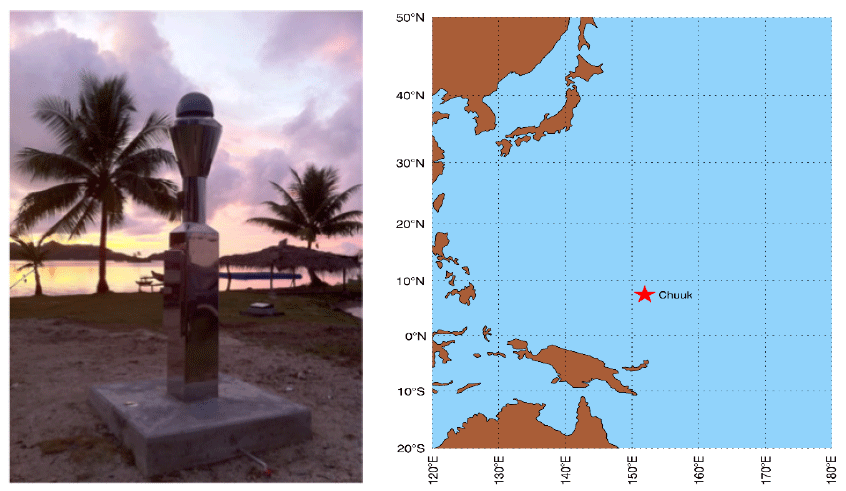
Fig. 1. Photograph (left) and geographic location map (right) of the KASI GNSS CHUK permanent site (Geographic: 7.5° N, 151.9° E; Geomagnetic: 0.4° N) at Chuuk in the Federated States of Micronesia.

Download Original Figure

The Korea Astronomy and Space Science Institute (KASI) has been operating a permanent geodetic Global Navigation Satellite System (GNSS) station in the Korea South Pacific Ocean Research Center of the Korea Institute of Ocean Science and Technology (KIOST). The station is located at Chuuk (Geographic: 7.5° N, 151.9° E; Geomagnetic: 0.4° N, site marker name: CHUK) in the Federated States of Micronesia. It is an ideal location to study the ionospheric characteristics of the EIA trough that have not been thus far observed. Fig. 1 shows the KASI CHUK GNSS site and its geographic location. This paper reports the first results in local time, monthly, and seasonal variations of GPS TEC, which had been continuously measured at this site during the solar maximum of 2014 with a high temporal resolution of 30 seconds. In Section 2, we briefly describe the method of GPS TEC measurement, and examine and discuss the seasonal and hourly variations of GPS TEC in Section 3. Finally, conclusions are given in Section 4.

2 GPS TEC MEASUREMENTS

The time delay of the radio signals from GPS satellites at an altitude of 20,200 km to ground-based GPS receivers is a result of their refraction by the total density of electrons along their path, which is defined as the slant TEC (STEC). The range delay, Δρ, can be obtained by the time delay of the radio signal using Eq. (1) (Liu & Gao 2004). The negative and positive signs are for carrier phase and pseudorange measurements, respectively.

Δ ρ = (ρ 1 − ρ 2) = ± 40.3 STEC f 2

(1)

The STEC is simply calculated from the diffrence in the range delay of GPS dual-frequency (f₁ = 1.57542 and f₂ = 1.22760 GHz) measurements as in Eq. (2), which can be derived using Eq. (1). Code pseudorange can provide biased measurement with unambiguous complete range, while carrier phase can provide relatively noise-free but integer cycle ambiguity and cycle slips. In this work, pseudoranges, ρ1₁ and ρ1₂ are smoothed with carrier phase measurements and are corrected with differential code bias to reduce range noise and instrument bias.

STEC= 1 40.3 f 12 f 22 f 22 − f 12 (ρ 1 − ρ 2) = 9.52 × 1016 (ρ 1 − ρ 2)

(2)

The vertical TEC (VTEC) is obtained from STEC using Eq. (3), in which R_e is the Earth radius, h_IPP is the height of ionospheric pierce point (IPP) or the height of peak electron density (hmF₂), and θ is the elevation angle of GPS satellites, assuming the single layer geometry model in which the ionosphere is a thin shell surrounding the Earth. The IPP is the point at which the line-of-sight from a satellite to a ground-based receiver intersects the shell. In this work, the h_IPP is assumed to be 325 km, based on the work of Yue et al. (2015) who used radio occultation measurements from Constellation Observation System for Meteorology, Ionosphere and Climate (COSMIC) to show that the hmF₂ is in the range of 300-350 km in the EIA trough.

VTEC = STEC 1 − (Re Re + h I P P cos θ) 2

(3)

The TEC values used in this work are the averaged values of VTEC, which are measured from satellites with the elevation angle of 45° or greater to reduce the errors caused by reflection from the ocean surface and large horizontal gradients of electron density in the EIA region. When h_IPP = 325 km and θ = 45°, the geomagnetic latitude of the measurement coverage is up to ~3.4° with the latitude range of the EIA trough between ~5° and ~20° that Yue et al. (2015) presented depending on local time and season. Considering the location of the EIA crest and the geometry for GPS TEC measurements, our observations can be considered to be representative of the characteristics of GPS TEC variation in the EIA trough.

3 RESULT AND DISCUSSION

3.1. The 27 Day Variations

The top and bottom plots in Fig.2 show the daily mean GPS TEC (TEC) values under geomagnetic quiet condtions (Kp ≤ 3.0) in the EIA trough measured at the KASI CHUK GNSS site, and F_10.7 index values for the solar extreme ultraviolet (EUV) flux in 2014, respectively. The daily TEC values show the 27 day trend according to the variations of the F_10.7 index, showing a clear contrast with summer. In general, the 27 day trends of ionospheric electron density may be effected by the planetary and tidal waves along with solar EUV flux variation according to the 27 day period of the solar rotation, as shown in the bottom plot of Fig. 2. According to Kim et al. (2008) who used altimetry TEC measurements from the Ocean Topography Experiment (TOPEX) satellite in the equatorial region to investigate the variations of the longitudinal wavenumber-4 (LW-4) structure of a non-migrating tide in the EIA, the amplitudes of LW-4 are < 20% in normalized TEC at a fixed longitude (90°, 200°, 270° and 360°) during periods of both low and high solar activities. Furthermore, the contribution of planetary waves to GPS TEC variation is known to be approximately < 10% (Borries et al. 2007). Considering the longitude (151.9° E) of the KASI CHUK GNSS site and the TEC amplitude of LW-4 and planetary waves, we ignored their contributions to the 27 day variation of daily TEC with the F_10.7 index of solar activity. Thus, further studies on the effects of planetary and tidal waves on monthly variation of GPS TEC are required. Because the contributions of tidal and planetary waves are excluded, the daily TEC patterns shown in the top plot of Fig. 2 represent only monthly variations according to variations of solar EUV flux corresponding to the 27 day period of the solar rotation along with a few ionospheric anomalies.

Fig. 2. The daily mean TEC values (solid circle) measured from the KASI CHUK GPS site and its fitting line (red line) and F_10.7 index under quiet geomagnetic condition (kp ≤ 3.0) in 2014.

Download Original Figure

3.2. Ionospheric Anomalies

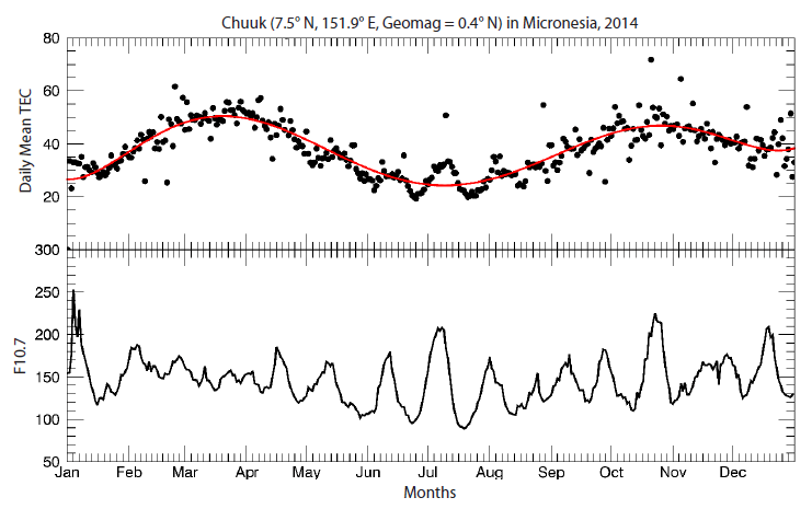
Fig. 2 suggests the occurrence of three anomalies in seasonal variation of the GPS TEC measurements at the KASI CHUK GPS site. The first anomaly occurs in the semi-annual variation, where the daily TEC in the equinoxes are greater than those in the solstices. The mechanism of anomaly is not clear at this time, but Fuller-Rowell (1998) proposed that the strong interhemispheric neutral wind in thermosphere contributes to decrease in O/N₂ ratio in F2 region during solstices, leading to decrease in the electron density (N_e) or TEC with the enhanced N₂. During equinoxes, thermospheric circulation between the northern and southern hemispheres weakens and O/N₂ ratio is higher than that of solstices. As a result, the semi-annual anomaly occurs, where N_e becomes higher during equinoxes than during solstices (Fuller-Rowell 1998; Rishbeth 1998; Lee et al. 2011). Zhao et al. (2007), using the NASA-JPL global TEC maps of year 2000, reported that amplitudes of semi-annual variation in the EIA trough region are in the range of ~15 % and ~35 % of the yearly average TEC. In the present work, amplitudes of semi-annual anomaly, which were determined through polynomial fitting and indicated with the red solid line in the top plot of Fig. 2, were 12.4 TECU (33 %) in 19^th of March and 8.8 TECU (23 %) in 25^th of October with a yearly average values of 38.0 TECU. Although the semi-annual variation of neutral composition by interhemispheric neutral wind in the thermosphere plays an important role in the development of this anomaly, Qian et al. (2013) suggest that changes of thermospheric composition and density are not practically sufficient to explain the amplitude variation of semi-annual anomaly.

The amplitude of the semi-annual variation was higher during the spring equinox than the autumn equinox, and this can be referred to as the equinox anomaly or equinoctial asymmetry where N_e is higher during the March equinox than that of the September equinox. However, the peak of daily TEC at the CHUK GNSS site occurred in October rather in September. The dominant factor causing the equinoctial asymmetry is usually considered to be thermospheric neutral wind (Rishbeth 1998). In case the solar EUV flux modulates the phase of equinoctial asymmetry, N_e during the September equinox may be higher than that of the March equinox, though (Unnikrishnan et al. 2002; Chen et al. 2012). Considering that the mean values of F_10.7 index were 149.3 (maximum = 182.2) and 151.2 (maximum = 224.8) during September and October, respectively, solar activity during these two months might produce the peak in October rather than in September. This implies that the variation of solar EUV radiation is an important factor that must be considered in investigating the phase modulation of equinoctial asymmetry in the EIA trough region. In addition, the contribution of thermospheric neutral wind and chemical composition according to solar activities must be considered.

Another important feature could be the annual anomaly where ionospheric plasma density is higher in December solstice than in June solstice in both of hemispheres or the winter anomaly where the daytime N_e is greater in winter than in summer in the mid-latitudes (Lee et al. 2011). However, it is difficult to identify the annual anomaly and the winter anomaly when we consider the latitude (7.5° N) of the KASI GNSS CHUK site. However, Liu et al. (2011) reported that winter anomalies can appear even at low latitudes in the north hemisphere based on COSMIC radio occultation measurements.

3.3. Local Time Variation

In order to investigate seasonal variations in the EIA trough in more detail, the scatter plot was generated based on the local time (LT = UT + 10 hour), as shown in Fig. 3. The annual, semi-annual, and equinox anomalies appear to be significantly affected by the variation in the solar flux between 08:00 and 18:00 LT. During daytime, the semi annual GPS TEC showed the maximum value in March and the second peak occurred in October; meanwhile, the magnitudes of two peaks were very weak after midnight and began to gradually increase only after 06:00 LT.

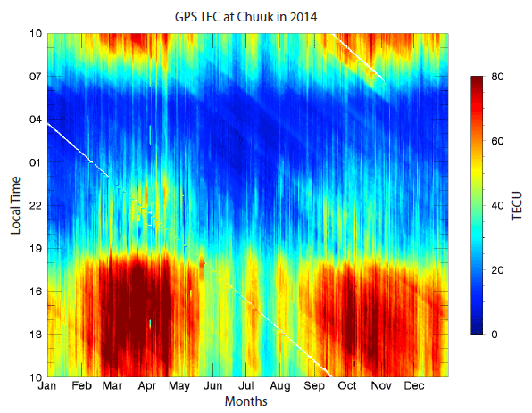
Fig. 3. Local time and seasonal variations of the mean VTEC values measured from the KASI CHUK GPS site during the solar maximum in year 2014.

Download Original Figure

Small GPS TEC enhancements were observed between 20:00 LT and 24:00 LT in the equinox in Fig. 3. The increase in nighttime GPS TEC during this period resembles features similar to those of the semi-annual variation during daytime. The increase in nighttime GPS TEC values before midnight could be explained by slow decrease in N_e from the high background N_e, which was developed during the daytime of equinox; however, GPS TEC values showed different behavior for the spring and autumn equinoxes. Considerable peaks appeared around 22:00-23:00 LT in the spring equinox, whereas the GPS TEC values continuously dropped during daytime in the autumn equinox. Tariku (2015) reported small enhancements of the GPS TEC between 21:00 and 23:00 LT during the spring equinox over low-latitude regions in the African sector during the period of the solar maximum (2012- 2013). He tried to explain the results with the combined effects of the slow decay time of the large background N_e with the pre-reversal enhancement (PRE) which is large vertical drift of plasma density at the equator during the spring equinox. According to this explanation, the nighttime TEC peaks during spring equinox, as shown in Fig. 3, might be a result of the mixed effects of the slow N_e decay time and high N_e production by the PRE. However, the contribution of the PRE to the enhancement of nighttime N_e in the EIA trough region is not clear at this time, and thus further research is required.

Zou et al. (2000) characterized annual and winter anomalies in the mid-latitudes, focusing on their nighttime features. They defined the winter anomaly as a condition of greater N_e in winter than in summer during daytime, while the anomaly disappears in the nighttime. They also defined the annual anomaly on a global scale as a condition of higher N_e in December than in June during both daytime and nighttime. In Fig. 3, the daily TEC in December is greater than that in June, and it shows the nighttime feature of annual anomaly reported by Zou et al. (2000). However, this could be attributed to the slow decay time of N_e with a high background N_e in December than in June. Furthermore, the increase or decrease in N_e due to thermospheric circulation of neutral wind and chemical composition should be investigated further using observational and modeling data.

4 CONCLUSIONS

The Korea Astronomy and Space Science Institute has operated the permanent geodetic GNSS site (KASI CHUK GNSS site) in cooperation with the Korea South Pacific Ocean Research Center of the Korea Institute of Ocean Science and Technology at Chuuk (Geographic: 7.5° N, 151.9° E; Geomagnetic: 0.4° N) in the EIA trough. This paper reports the results of the first observations of ionospheric trends using mean VTEC values which were measured from satellites with the elevation angle of 45° or greater at the KASI CHUK GNSS site during the solar maximum in 2014. The horizontal coverage of observation was up to about 3.5° within the EIA trough.

Daily mean TEC values showed variations corresponding to the 27 day period of the solar rotation; this trend showed a clear contrast in summer. The seasonal variation of daily mean TEC exhibits the combined features together with the semi-annual anomaly, the equinoctial asymmetry, and the annual anomaly. The semi-annual anomaly had the amplitudes of 12.4 TECU (33 %) on March 19 and 8.8 TECU (23 %) on October 25, with a yearly average value of 38.0 TECU. An equinox asymmetry was also observed; the March equinox has higher amplitude than the October equinox, as shown by the daily mean TEC variation. The last anomaly feature reflected the annual anomaly where the daily mean TEC values were higher in December than in June.

The annual/semi-annual anomaly and equinoctial asymmetry may be explained by the significant effects of the solar flux variation between 08:00 and 18:00 LT. During daytime, the first and second peaks of the semi-annual anomaly occurred in March and in October, respectively. It disappeared after midnight and began to gradually develop after 06:00 LT. The nighttime GPS TEC enhancements between 20:00 LT and 24:00 LT similarly exhibited the semi-annual variation during daytime. Considerable peaks appeared around 22:00- 23:00 LT in the spring equinox, whereas the GPS TEC values continuously decreased during daytime in the autumn equinox. The nighttime TEC enhancement between 22:00- 23:00 LT in the spring equinox could be attributed to the mixed effect of the slow N_e loss time and other N_e production mechanisms such as the PRE during the spring equinox.

The ionospheric anomaly originally indicates any departure from the solar-controlled ionospheric behavior, and many research topics have retained its physical mechanism and effects of GPS radio signals. Ionospheric storms, which may cause degradation of GPS abilities, might develop more vigorously under ionospheric anomalies according to solar and geomagnetic activities (Mendillo 2006; Rishbeth & Müller-Wodarg 2006). For further works, we will examine the relationships between the accuracy of GPS positioning and ionospheric storm occurrences according to the variations in ionospheric anomalies with seasonal patterns of GPS TEC in LT.

ACKNOWLEDGMENTS

This work is funded by the project of space geodesy infrastructure management and its application of Korea Astronomy and Space Science Institute (KASI) in 2015. We are thankful to the personnel of Korea South Pacific Ocean Research Center (KSORC) of Korea Institute of Ocean Science and Technology (KIOST) for their support in mounting the geodetic permanent GNSS station at Chuuk in the Federated States of Micronesia. The F_10.7 index data were obtained from OMNI website (http://omniweb.gsfc.nasa.gov).

References

Arunpold S, Tripathi NK, Chowdhary VR, Raju DK. Comparison of GPS-TEC measurements with IRI-2007, and IRI-2012, modeled TEC at an equatorial latitude station, Bangkok, Thailand. J. Atmos. Sol.-Terr. Phys. 2014; 117:88-94.

Bagiya MS, Joshi HP, Iyer KN, Aggarwal M, Ravindran S , et al. TEC variations during low solar activity period (2005,-2007,) near the equatorial ionospheric anomaly crest region in India. Ann. Geophys. 2009; 27:1047-1057.

Borries C, Jakowski N, Jacobi Ch, Hoffmann P, Pogoreltsev A. Spectral analysis of planetary waves seen in ionospheric total electron content (TEC): first results using GPS differential TEC and stratospheric reanalyses. J. Atmos. Sol.-Terr. Phys. 2007; 69:2442-2451.

Chen Y, Liu L, Wan W, Ren Z. Equinoctial asymmetry in solar activity variations of NmF2 and TEC. Ann. Geophys. 2012; 30:613- 622.

Chung JK, Choi BK. Statistics of ionospheric storms using GPS TEC measurements between 2002, and 2014, in Juju. Korea. J. Astron. Space Sci. 2015; 32:335-340.

Fuller-Rowell TJ. The “thermospheric spoon”: a mechanism for the semiannual density variation. J. Geophys. Res. 1998; 103:3951-3956.

Jee G, Lee HB, Kim YH, Chung JK, Cho J. Assessment of GPS global ionosphere maps (GIM) by comparison between CODE GIM and TOPEX/Jason TEC data ionospheric perspective. J. Geophys. Res. 2010; 115:A10319.

Kim E, Jee G, Kim YH. Seasonal characteristics of the longitudinal wavenumber-4 structure in the equatorial ionospheric anomaly. J. Astron. Space Sci. 2008; 25:335-346.

Lee WK, Kil H, Kwak YS, Wu Q, Cho S , et al. The winter anomaly in the middle-latitude F region during the solar minimum period observed by the Constellation Observing System for Meteorology, Ionosphere, and Climate. J. Geophys. Res. 2011; 116:A02302.

10.

Liu L, Le H, Chen Y, He M, Wan W , et al. Features of the middle- and low-latitude ionosphere during solar minimum as revealed from COSMIC radio occultation measurements. J. Geophys. Res. 2011; 116:A09307.

11.

Liu Z, Gao Y. Ionospheric TEC predictions over a local area GPS reference network. GPS Solut. 2004; 8:23-29.

12.

Mendillo M. Storms in the ionosphere patterns and processes for total electron content. Rev. Geophys. 2006; 44:RG4001.

13.

Qian L, Burns AG, Solomon SC, Wang W. Annual/semiannual variation of the ionosphere. Geophys. Res. Lett. 2013; 40:1928-1933.

14.

Rishbeth H. How the thermospheric circulation affects the ionospheric F2-layer. J. Atmos. Sol.-Terr. Phys. 1998; 60:1385-1402.

15.

Rishbeth H, Muller-Wodarg ICF. Why is there more ionosphere in January than in July? The annual asymmetry in the F2- layer. Ann. Geophys. 2006; 24:3293-3311.

16.

Skone S, Coster A. Studies of storm-enhanced density impact on DGPS using IGS reference station data. J. Geod. 2009; 83:235- 240.

17.

Tariku YA. Patterns of GPS-TEC variation over low-latitude regions (African sector) during the deep solar minimum (2008 to 2009) and solar maximum (2012 to 2013) phases. Earth Planets Space. 2015; 67:35.

18.

Tsai HF, Liu JY, Tsai WH, Liu CH, Tseng CL , et al. Seasonal variations of the ionospheric total electron content in Asian equatorial anomaly regions. J. Geophys. Res. 2001; 106:30363- 30369.

19.

Unnikrishnan K, Nair RB, Venugopal C. Harmonic analysis and an empirical model for TEC over Palehua. J. Atmos. Sol.-Terr. Phys. 2002; 64:1833-1840.

20.

Yue X, Schreiner WS, Kuo YH, Lei J. Ionosphere equatorial ionization anomaly observed by GPS radio occultations during 2006-2014. J. Atmos. Sol.-Terr. Phys. 2015; 129:30-40.

21.

Zhang V, Li Z. Measured ionospheric delay correction for codebased GPS time transfer. Proceedings of the 46th Annual Precise Time and Time interval Systems and Applications Meeting. 2014, Boston, Massachusetts; 1-4 Dec 2014.

22.

Zhao B, Wan W, Liu L, Ren Z. Characteristics of the ionospheric total electron content of the equatorial ionization anomaly in the Asian-Australian region during 1996-2004. Ann. Geophys. 2009; 27:3861-3873.

23.

Zou L, Rishbeth H, Muller-Wodarg ICF, Aylward AD, Millward GH , et al. Annual and semiannual variations in the ionospheric F2-layer I Modelling. Ann. Geophys. 2000; 18:927- 944.