


1 INTRODUCTION
IPS-driven ENLIL model was jointly developed by University of California, San Diego (UCSD) and National Aeronaucics and Space Administration/Goddard Space Flight Center (NASA/ GSFC) and this model has been in operation by Korean Space Weather Cetner (KSWC) since 2014. It provides 3-day forecasts and crucial information for solar wind researches (Jackson et al. 2015; Yu et al. 2015). The basic model of IPS-driven ENLIL model is the ENLIL model; the ENLIL model is a simulation model to numerically solve physical equations using solar wind information in the region close to the Sun (0.1 AU) to calculate the progression of solar wind (Odstrčil & Pizzo 1999a, 1999b; Odstrčil 2003). As a solar wind prediction model, it is utilized in space weather forecasts in Space Weather Prediction Center (SWPC), Bureau of Meteorology (BOM), and Meteorological Office (Met Office). The existing ENLIL model utilizes the results of the Wang-Sheeley-Arge (WSA) model as input data at the distance of 0.1 AU. However, in this model, when coronal mass ejection (CME) occurs, the operator should analyze the coronagraph satellite data to obtain such information at the time of occurrence, location, velocity, angular width, and should provide those into the model in person. In order to address this inconvenience, IPS-driven ENLIL model utilizes IPS tomography model results instead of WSA model results to enable automated analysis of CME to obviate the analysis by the operator himself. IPS (Inter-planetary Scintillation) refers to the method to estimate the velocity and the density in the interplanetary space around the Sun by measuring scintillation of signals from radio source (e.g., radio galaxy) located in the rear side of the Sun and analyzing those series of observation data. This model is also referred to as the IPS tomography model since it diagnoses the physical state of the location of interest by collecting line of sight information from these observation data (Jackson et al. 2013). The purpose of solar wind analysis using the IPS tomography is to find out the distribution of velocity and density for the space around the Sun, thus, it could be a kind of solar wind prediction model. Currently, IPS observations have been made in Japan, Australia, Mexico, and India besides our country. Since IPS observations are possible during daytime only, joint effort to improve IPS observation accuracy by integrating observation data of various longitudes are in progress (Bisi et al. 2016).
In this study, in order to enhance the prediction capability of IPS-driven ENLIL model, in addition to improving the IPS tomography data which are based on observations, selection of the best combinations of free parameters to give optimal model results is attempted by analyzing the free parameters which are necessary to run the ENLIL model. The free parameter of ENLIL model consists of the values of magnetic field, density, temperature, and velocity, which represents ambient physical quantities in interplanetary space. And the final model results strongly depend on the combinations of these free parameters which set the initial values of physical quantities of interplanetary space. Hence, it is crucial to find the combination of these free parameters giving best prediction to improve the prediction accuracy of ENLIL model. Currently, the IPS-driven ENLIL model which is in operation in KSWC utilizes arbitrary values of parameters and prediction performance of the model can be improved significantly by using the combination of parameters obtained through this research.
2 METHODS
There are four kinds of free parameters utilized in IPS-driven ENLIL model. These parameters correspond to the ambient magnetic field, ambient density, ambient temperature, and ambient velocity, respectively. Also, the variable names in the model are ‘ambb’, 'ambd', 'ambt', and ‘ambv’, respectively and the free parameters have the following names and values given in Table 1. The names of variables are designated according to the input values of each parameter and the magnitude of scaling factor in compliance with the rules specified by the model developer. These free parameters were selected since these are the most basic physical quantities in interplanetary space. And they are related to solar wind speed and density most closely. Thus, the possible number of combinations based on these free parameters is 1440 and the results of the model are summarized for selected periods.
Four analysis periods were selected for model execution: Kp index less than 4, interplanetary magnetic filed (IMF) Bz less than ±5 nT, solar wind speed less than 450 km/s, and quiet for 7 days (Table 2). The solar wind speed and density data of the solar wind electron proton alpha monitor (SWEPAM) data obtained from the advanced composition explorer (ACE) satellite were used for comparison with the results of the model. Also, root-mean-square error (RMSE) and prediction efficiency (PE) methods were used for statistical analysis of the comparison results between the model and the observed. Through this statistical analysis of integrated data for 4 analysis periods, best combinations of parameters were determined to predict density and velocity.
3 RESULTS
Table 3 shows the top 10 combinations of free parameters selected from 1,440 combinations for 4 analysis periods through RMSE and PE.
According to the analysis of the top 10 combinations, the results of RMSE and PE showed consistency each other. It was found that b00 is placed at a higher rank than b10 for ambient magnetic fields and that for ambient density, d20 and d30 are dominant in the high ranks; for ambient temperatures, s20~t25 parameters are ranked higher; for ambient velocity, all the top 10 combinations include w150 in common.
For the trend analysis of input variation for each free parameter, comparison results were plotted for the earliest analysis period (2015.04.24.00 UT ~ 2015.05.01.00 UT). As a reference data, the results of the top rank combination of d20s30w150 were selected and comparison was made for the results of b00 and b10 inputs which indicate the existence of magnetic field.
Fig. 1 shows a comparison plot of ambient density changes; ambient temperature and ambient velocity were fixed at s30w150. We can find that when the magnetic field factor is zero (b00), the results of density and velocity from the model increases as ambient density increases and in the other case (b10), as ambient density goes lower, the impact of magnetic field becomes larger changing the trend of the curve.
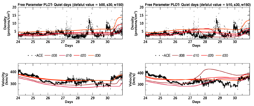
Fig. 2 shows a comparison plot for ambient temperature changes; ambient density and ambient velocity were set to d20w150. In general, the trend showed that as ambient temperatures increase, model velocities get faster and as ambient temperatures decrease, densities go lower. Also, when the magnetic field factor is applied, it was found that the lower the ambient temperatures are, the larger the impact of the magnetic field is.
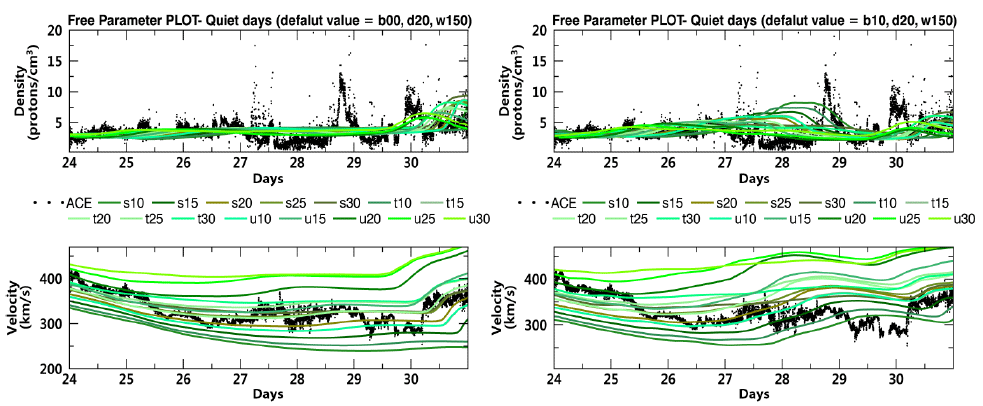
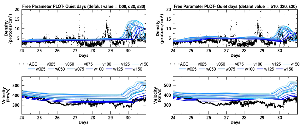
Fig. 3 is a comparison plot for ambient velocity changes; ambient density and ambient temperature were fixed at d20s30. In the model, since ambient velocity takes the role of reduction (Table 1), the velocity of the model is the fastest for v025 or w025 and gradually gets slower as it come down to v150 or w150. It is noteworthy that magnetic field factor has little impact on the result unlike the plot of ambient temperature and ambient density changes.
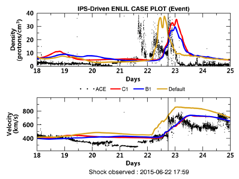
In order to find out the model performance improvement by applying the selected combination of free parameters, verification was performed for quiet periods and an event period. For the quiet periods, two additional analysis periods were selected with the same condition of analysis periods selected for free parameter combination analysis. The event period selected was the period of actual CME occurrence with the G4 alarm issued; it happened on 02 UT, June 21, 2015 and CME shock was first observed by ACE satellite on 18 UT, June 22, 2015 (Table 4). In this event period, while multiple CME events have occurred, the verification was performed based on the shock which actuated G4 (Kp=8) alarm. The time when the shock reached the Earth was obtained from the records of “CME Arrival Time Scoreboard” in CCMC (CCMC 2016).
| Parametars | Period |
|---|---|
| Quiet-1 | 2015.01.12.00 UT ~ 2015.01.19.00 UT |
| Quiet-2 | 2016.02.22.00 UT ~ 2016.02.29.00 UT |
| Event (G4) | 2015.06.18.00 UT ~ 2015.06.25.00 UT (Shock Arrival : 2015.06.22.17:59 UT) |
The free parameter combinations selected for verification are b00d20s30w150 (Rank 1) and b10d20s30w150 (Rank 58) which is the highest rank with the magnetic field factor. And the model performance was verified by comparing the results with those of existing typical combination. The details of the existing free parameter combination and the selected combinations are shown in Table 5.
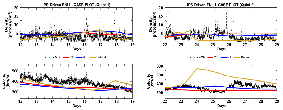
Fig. 4 shows the comparison results of the model outputs for quiet periods. The RMSE analysis was performed to evaluate the improvement in prediction performance quantitatively (Table 6). For these two periods, generally better model performance was observed and in case of Quiet-2 particular, the results of Default were very bad and the results of C1 were better than those of B1. Thus, it was verified that the free parameter combinations selected in this study results in better performance than the existing free parameter combination (default).
| parameter sets | RMSE_density | RMSE_velocity | |
|---|---|---|---|
| Quiet-1 | C1 | 2.4150 | 50.4522 |
| B1 | 2.8255 | 61.8336 | |
| Default | 2.5397 | 53.3159 | |
|
|
|||
| Quiet-2 | C1 | 3.4986 | 44.4785 |
| B1 | 3.2845 | 36.8176 | |
| Default | 3.8944 | 125.3921 | |
Fig. 5 shows the verification result for the event period. Unlike quiet periods, since the prediction of the Earth arrival time and the scale of CME shock is important for event periods, it is not suitable to use the RMSE method, thus, the peak of the graph was compared directly. When the CME shock arrives, the solar wind speed and density of ACE observation data increases at the same time. Since there were multiple events in this period, we can verify the arrival of more than one shock. However, due to the characteristics of IPS observation, observation was made for one big CME united and it was assumed that the results of C1 and B1 are observation results for the same CME of the same scale. Also, the reference time was decided at the time of shock arrival which actuated G4 alarm. According to the previous model, it was estimated that the time of increase in density was 03 UT, June 22 which was 15 hr ahead of actual shock arrival time. However, after the application of C1 and B1 combinations of free parameters, it was predicted that the time of shock arrival fell on 13 UT, June 22, which shows only 5 hr difference compared to the actual results. In other words, with the application of free parameter combination selected through this study, the Earth arrival time of CME shock can be more accurately predicted than the existing model.
4 DISCUSSION AND CONCLUSION
In this paper, in order to improve the prediction performance of the IPS-driven ENLIL model which has been utilized in the area of forecasts and researches of solar wind, the combinations of free parameters showing best prediction performance were determined through statistical analysis and the characteristics of those best combinations were analyzed. In addition, the variations of model results according to the changes of free parameters were analyzed and a measure to apply those best combinations to the model was set up. Finally, the application results of those selected combinations of free parameters of the model turned out to show improved performance for a quiet period and an event period. Especially, in the event period, the predicted results of best combinations were found to be significantly closer to the actual CME arrival time than those of the existing model. In general, the ENLIL model which is the basic model of IPSdriven ENLIL mode, predicts that CME arrives about 6~7 hr earlier than the actual arrival of the CME statistically (Taktakishvili et al. 2009; Mays et al. 2015). However, it is expected to resolve this issue of the existing ENLIL model through the application of the free parameter combinations determined in this study.
Meanwhile, the free parameters used in the analysis allow arbitrary input values other than fixed values, that is, each free parameter allows floating point input and there is no restriction on scaling factors enabling an unlimited number of combinations actually. Also, while the current input data of IPS-driven ENLIL model are based on observations of Nagoya in Japan, researches of free parameter values are necessary in case multiple input data are utilized according to the study of the IPS tomography model enhancement. However, when we take into account the characteristics of top ranked combinations analyzed in this study and analysis results of model behavior due to the variation of free parameter values, it is expected to find the free parameter combination of enhanced performance. For further study, it is expected to improve forecast performance of the solar wind by verifying the results in additional CME event periods and applying those to IPS-driven ENLIL model.