1 INTRODUCTION
Spacecraft formation flying has several advantages such as flexible configurations of formations with respect to space missions, and practicable costs for production and launches. Moreover, there have been significant contributions to the field of space missions (Tapley et al. 2004; Krieger et al. 2007). Precise relative navigation (orbit estimation) that provides the relative position and velocity of each spacecraft with respect to the other is an essential part of spacecraft formation flying missions. Recently, significant attention was attracted by a laser instrument, given that it can precisely measure the relative distance between spacecrafts in formations (Shaddock 2008; Wang et al. 2011; Sheard et al. 2012). The precise measurement of the relative distance can help improve the performance of relative navigation. Numerical simulations by Jung et al. (2012) revealed that the relative navigation for a pair of spacecrafts with consecutive laser-based measurements using the extended Kalman filter (EKF) could determine the relative position with errors at the millimeter-level at a relative distance of 10 km, and errors at the sub-millimeter level at a relative distance of 1 km. However, consecutive measurements require that a laser mounted on a spacecraft in formation is precisely aimed at a target spacecraft. Otherwise, particularly in cases where the relative distance between the spacecrafts in formation is very long, measurement failure may occur if the other spacecraft is not targeted. It is therefore necessary to develop a relative navigation strategy for satellites flying in formation when laser measurements are intermittent.
Recently, there have been discussions on the relative navigation for spacecraft formation flying using intermittent laser-based measurement data (Lee et al. 2017; Lee et al. 2018). Lee et al. (2017) developed a relative navigation algorithm that uses the least squares recursively with intermittent measurements, which is referred to as a least squares recursive filter (LSRF)-based relative navigation algorithm in this paper. Lee et al. (2017) confirmed the degradation of the performance of the EKF-based relative navigation algorithm when measurements were carried out intermittently, and compared the performances of the EKF- and LSRF-based relative navigations. However, it was assumed that laserbased measurement data were obtained at 10 Hz; thus, an unscented Kalman filter (UKF)-based relative navigation algorithm with intermittent measurements was developed, and the performances of the EKF- and UKF-based relative navigations were compared. In this study, numerical simulations of the EKF-, UKF-, and LSRF-based relative navigations were conducted for a pair of spacecrafts; namely, chief and deputy spacecrafts, with intermittent laser-based measurements. The simulation results were then analyzed. Thereafter, the most appropriate algorithm among the EKF- , UKF-, and LSRF-based algorithms for real-time relative orbit estimation with intermittent measurements was determined by comparing the esti-mation accuracies and the computation times required for the estimations.
The remainder of the paper is organized as follows. In Sections 2 and 3, the dynamic model and laser-based measurement are introduced, respectively. The relative navigation algorithms are discussed in Section 4. In Section 5, the results of the relative navigation simulations are presented, followed by the conclusions and directions for future work in Section 6.
2 DYNAMIC MODEL
In this study, a precise relative navigation algorithm with a precise dynamic model was developed for spacecrafts in low earth orbits (LEOs) using the two-body equation with the appropriate perturbations added, as expressed by Eq. (1):
where μE represents the standard gravitational parameter of the Earth; represent the absolute position and acceleration vector of a spacecraft in the earth-centered inertial (ECI) frame, respectively; and represent perturbations due to the aspherical properties of the Earth, air drag, gravitational forces from the Sun and Moon, and solar radiation pressure, respectively., Moreover JGM3 and the exponential model were employed for , respectively. For , reference was made to Vallado (2013) and Jung et al. (2012). The absolute orbit (or absolute state vector) o fthe spacecraft consists of the position and velocity, which are represented in the ECI frame, as expressed by Eq. (2):
where x, y and z are positions in the x-, y-, and z- axis in the ECI frame, respectively; and are the rates of x, y, and z, respectively. The absolute orbit can be propagated by integrating Eq.(1).
This study considers two spacecrafts. Thus, the propagation of the relative, and can be achieved by obtaining the difference between the two propagated absolute orbits of the chief and deputy in the ECI frame. The measurement data consists of the relative range and attitude angles in the spherical frame that originates at the center of mass of the chief, the relative orbit, or the relative state vector; which is represented in the spherical frame as , and defined in Eq.(3):
where ρ is the relative range; θ (azimuth) and ϕ (elevation) are the relative angles of the deputy with respect to the chief; and are the rates of ρ, θ, and ϕ, respectively. A detailed descriptions of the transformation from the ECI frame to the spherical frame can be found in Jung et al.(2012).
3 LASER-BASED MEASUREMENT
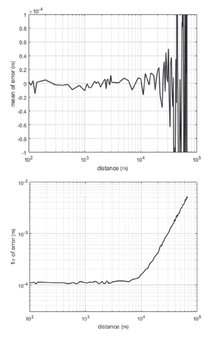
The measurement data for the relative navigation consists of the relative range (ρ) measured by a femtosecond laser and relative angles, namely, the azimuth (θ) and elevation (ϕ) between the two spacecrafts. The relative range can be produced by the femtosecond laser system, as described by Jang et al.(2014). The laswer system is mounted on the fief spacecraft and operated by the principle of synthetic wavelength interferometry. In this study, the measurement value of the relative range from the laser system was evaluated using software that simulates a system was evaluated using software that simulates a femtosecond laser. Fig.1 presents the measurement performance of the laser that is described by the mean and standard deviation of the measurement error with respect to distance. The mean and standard deviation of the error with respect to distance. The mean and standard deviation of the error diverges after approximately 10km; thus, 10km is the distance limit of the femtosecond laser (Kang et al.2017).
The relative angles of the deputy, with respect to the chief, that correspond to a laser direction were assumed to be obtained via the attitude determination of the chief. In this study, the uncertainty of the attitude determination was discussed instead of the algorithm of the attitude determination. This uncertainty, represented by Gaussian random errors with a zero mean and a standard deviation of a certain value, was added to the true azimuth and elevation (Jung et al. 2012). These values, with the Gaussian random errors added, were assumed to be the measurement values of the relative attitude angles.
4 RELATIVE NAVIGATION ALGORITHMS
Consider a nonlinear discrete-time system that consists of the dynamic and measurement models as expressed in Eqs. (4) and (5):
where represent a state vector and measurement vector, respectively. The subscript represents a time step. The constants n and m are dimensions of the state and measurement vectors, respectively; and the nonlinear function f and hk are the dynamic and measurement models of the system, respectively. The vectors denote a provess nnoise and a measurement noise with their respective error coveriance matrices Q and R. The process noise and measurement noise were assumed to be additive and uncorrelated.
The absolute orbits of the chief and deputy consist of the positioni and velocity, as represented in the ECI fame: are propagated by integrating Eq. (1). A nonllinear discrete-time system with Eq. (1) is expressed by Eq. (6):
where f is the two-body equation with perturbations added, as expressed by Eq.(1). By subtracting the two propagated absolute orbits , the propagated relative orbit represented in the ECI fame can be calculated as expressed in Eq.(7):
Transforming the ECI frame into a spherical frame allows the propagated relative orbit represented in the spherical frame to be obtained (Jung et al. 2012, Lee et al. 2015).)
The measurement model hk is as described in Eq. (8):
As seen in Eq. (8), the measurement model hk is the time invariant linear H. The relative orbit and the measurement data ρ, θ, and ϕ are represented in the spherical frame; thus, the measurement model H is [I3x3 03x3]. Adding the scale factor sf to H eliminates the drift due to the relative distance rate (Jung et al. 2012).
The EKF is a real-time estimator that approximates the state vector of an object as a Gaussian random variable (GRV), and determines the best estimate of the state vector using measurement data in systems where both the dynamic model and sensor contain uncertainties (i.e., process noise and measurement noise). The EKF contains the two fundamental components: prediction and correction. The prediction component propagates the estimates of the state vector and error covariance matrix at a previous time step to obtain the predicted state vector and error covariance matrix at the current time step. The correction component corrects the predicted state vector and error covariance matrix using the measurement data and Kalman gain. These corrected values are the estimated state vector and error covariance matrix at the current time step. The detailed algorithm and equations of the EKF can be found in Vallado (2013). In the EKF, the mean of the state vector is propagated through a first-order linearized nonlinear system. If measurement data are consecutively available, the EKF can appropriately approximate a nonlinear system. Otherwise, the first-order linearization can induce estimation errors. In addition, if the initial error or the nonlinearity of the system increases, the EKF can provide suboptimal estimations (Lee & Alfriend 2003).
In this study, the relative navigation for spacecraft formation flying with intermittent laser-based measurements was addressed. In previous studies that considered relative navigation using a femtosecond laser, it was assumed that measurements were carried out consecutively. Thus, the estimation algorithms in these studies based on the EKF implemented continuous prediction and measurement corrections (Jung et al. 2012; Lee et al. 2015; Oh et al. 2016). However, it is possible for measurement data to not be obtained consecutively due to failure in inter-spacecraft alignment, particularly in cases when the distance between spacecrafts is large. When there is no measurement data, measurement correction cannot be implemented. Therefore, if laser-based measurement data are available at a certain instant k in this study, both prediction and measurement corrections are implemented; otherwise, only the prediction correction is implemented.
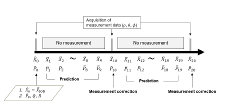
Fig. 2 reveals how the EKF-based relative navigation algorithm with intermittent laser-based measurements is implemented. In the figure, represent the predicted state vector, namely, the predicted relative orbit and error covariance matrix, respectively; and represent the estimated relative orbit and error covariance matrix, respectively. As can be seen in Fig. 2, the initial relative orbit by the initial orbit determination (IOD) is set to the estimated relative orbit at the initial time step . The relative navigation is then implemented. If laser-based measurement data are available for ρ, θ, and ϕ, prediction and measurement corrections are implemented. Otherwise, only the prediction correction is implemented.
The UKF is also a real-time estimator that can determine the best estimate of the state vector of an object using measurement data in systems where both the dynamic model and sensor contain uncertainties. Both the EKF and UKF approximate a state vector as a GRV. However, unlike the EKF, the UKF represents the Gaussian distribution of the state vector using sigma points based on unscented transformation (UT). The UKF propagates sigma points using a true dynamic model of a nonlinear system; thus, the UKF can accurately propagate the mean and corresponding error covariance matrix of the state vector to the 3rd order in the Taylor series expansion for all nonlinearities (Wan & Van Der Merwe 2000).
The distribution of sigma points is determined by the scaling parameters α, β, κ, and λ. Moreover, α affects the distribution of the sigma points around the mean of the GRV; β is used to incorporate prior knowledge of the distribution of the GRV; κ is a secondary scaling parameter; and λ is determined by λ=α2(n+κ)−n, where n is the dimension of the state vector (Wan & Van Der Merwe 2000; Kim et al. 2011). The filtering performance of the UKF, such as the accuracy and convergence in estimation, are significantly reliant on scaling parameters. Therefore, setting scaling parameters is a major issue when using UKF. Moreover, α is usually set as a small positive value such as 0≤α≤1. In Section 5, several navigation results that depend on α are presented; β=2 is optimal for Gaussian distributions; and κ is typically set as 0 or 3−n (Wan & Van Der Merwe 2000; Kim et al. 2011). In this study, κ=3−n was used to minimize the difference between the moments of the standard Gaussian distribution and the sigma points up to the fourth order (Julier et al. 2000). The detailed algorithm and equations of the UKF can be found in Wan & Van Der Merwe (2000).
The UKF is a type of Kalman filter, similar to the EKF. In other words, if laser-based measurement data are available at a certain instant k, both prediction and measurement corrections are implemented. Otherwise, only the prediction correction is implemented. Fig. 2 presents the implementation procedure of UKF-based relative navigation with intermittent laser-based measurements.
The least squares method is a post-processing estimator for the state vector of an object. It determines the best estimate of a state vector at a given instant that minimizes the sum of the square of residuals between the measurement data and computed measurement data, which is carried out using a measurement model. As a post-processing estimator, the least squares method uses an entire set of measurement data within a given time-period. In this study, the nonlinear weighted least squares method was used. The nonlinear weighted least squares method can estimate a state vector in nonlinear systems by linearizing a system, obtaining an approximate solution, and iteratively refining the approximated solution (Vallado 2013). This iterative refining process is called “differential correction.” The detailed algorithm and equations of the least squares can be found in Vallado (2013).
In this study, a relative navigation algorithm was employed using least squares recursively. This algorithm was proposed by Lee et al. (2017) to solve the degradation problem of the EKF-based algorithm, and is termed the LSRF-based relative navigation algorithm in this paper. Before implementing the LSRF-based relative navigation algorithm, a fixed time interval must be defined to obtain measurement data. It was assumed that a laser-based measurement outage period was fixed and could be determined. A fixed-time interval was therefore set to obtain measurement data equal to the measurement outage period. Hereinafter, the ratio of the fixed-time interval to obtain measurement data equal to the measurement outage period is referred to as the “window size”. Moreover, the window size was 1. The period for the estimation of the relative orbit through the LSRF-based relative navigation algorithm was set to a product of the window-size and measurement outage period. Thus, the window-size is an indicator of how many measurement data sets are used in the relative navigation.
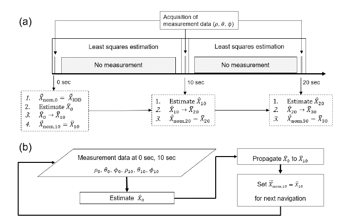
Fig. 3 illustrates the implementation of an LSRF-based relative navigation algorithm with intermittent laser-based measurements. Following the determination of the initial relative orbit , the navigation for the relative orbit commences. At the initial time step (k=0), the LSRF-based algorithm set as a nominal relative orbit . For example, it is assumed that measurements could be made at the initial time step and at fixed 10 sec intervals. The window-size is 1; thus, navigation using measurement data at 0 sec and 10 sec is carried out at 10 sec. The LSRF-based algorithm propagates to calculate the relative orbits at 10 sec () and the computed measurement data that correspond to the relative orbits at 0 sec and 10 sec. Then, using measurement data at 0 sec and 10 sec (), the algorithm calculates the measurement residual and the partial derivative matrix A of the least squares. With and A, the correction vector for the initial nominal relative orbit can be calculated using the normal equation of the least squares. Thereafter, can be updated to by adding . The iterative differential correction for the initial relative orbit stops if the root-mean-square of the residual matrix remains constant within a given tolerance, which was set to 5×10⁻⁸ in this study. Satisfying the stopping criterion means that the least squares finds the best estimate of the relative orbit at the initial time step . If the stopping criterion is not satisfied, the least squares restarts with updated relative orbits . In the next process, the algorithm propagates to time step 10 sec. The propagated relative orbit at 10 sec is set to the nominal relative orbit of the next navigation process at 20 sec. At 20 sec, the algorithm finds the best estimate of the relative orbit at 10 sec () using measurement data at 10 sec and 20 sec (). The algorithm then propagates to and sets as for the next navigation process at 30 sec. The LSRF-based relative navigation algorithm with intermittent laser-based measurements is implemented over the simulation time-period in this recursive manner.
5 NUMERICAL SIMULATIONS AND ANALYSES
Numerical simulations were implemented to analyze and compare the performances of the three relative navigation algorithms based on EKF, UKF, and LSRF for spacecraft formation flying with intermittent laser-based measurements. The simulations considered two spacecrafts; namely, chief and deputy spacecrafts that orbit the Earth, forming a projected circular orbit (PCO). The chief at an altitude of 613 km is assumed to have a circular orbit around the Earth at an inclination of 97.8 °. The initial radius of the PCO was set as 10 km, given that the distance limit of the femtosecond laser is 10 km. It was assumed that the chief was equipped with the femtosecond laser instrument, and the deputy had a reflector mirror to return the laser signal.
The true orbits of the chief and deputy were determined by the numerical integration of the dynamic model based on Eq. (1). For the true orbits, the perturbation was driven by the unknown acceleration of magnitude 10-14 m/s2, which was added to Eq. (1) as described in Eq. (9), given that the true orbits can never fully be known (Jung et al. 2012).
Eq. (9) considers the aspherical property of the Earth of degree and order 20×20. The dynamic model for the relative navigation algorithms is the two-body equation with the added gravitational perturbation derived from the aspherical property of the Earth of degree and order 2×0, as described in Eq. (10), to reduce the computational load for real-time navigation.
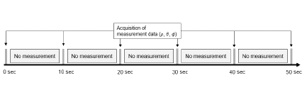
In cases where a laser mounted on the chief in formation is precisely aimed at the deputy, laser-based measurement data are consecutively obtained. However, this study addresses the relative navigation with intermittent measurements, under the assumption that the targeting of the deputy is not always guaranteed, due to the large relative distance. In this study, the laser-based measurement outage period was assumed to be constant throughout the simulation. For example, if the outage period is set as 10 sec, laser-based measurement data would be obtained in 10 sec intervals during the simulation (see Fig. 4). Simulations with different measurement outage periods were implemented to determine the influence of intermittent laser-based measurements on the relative navigation.
The simulation time was set as 6,000 sec, and the uncertainty of the attitude determination of the chief was assumed to be 0.001 ° for every simulation.
Given that the scaling parameters within the UKF significantly influence the estimation performance, the simulations of the relative navigation of the UKF-based algorithm were implemented in advance, while adjusting the scaling parameters. The influence of α is more significant than that of β, κ, and λ; thus, only α was adjusted, and the remaining parameters were set as β=2 and κ=3−n (Lee et al. 2018). Moreover, λ was determined by 3α2−6 (Wan & Van Der Merwe 2000). The initial relative orbit was obtained by adding the IOD error to the true orbit, and the following are the conditions of simulation case 1. The IOD errors correspond to a relative position and velocity of approximately 20 m and 20 cm/s between the chief and deputy, respectively. The initial error covariance matrix P0 was defined as expressed in Eq. (11):
where M2error is a diagonal matrix in which the diagonal entries correspond to the IOD error. Moreover, Q and R were empirically determined to improve the relative navigation performance. Fig. 5 presents the various navigation errors while adjusting α for simulation case 1. The numbers in the legend in Fig. 5 denote the measurement outage period.
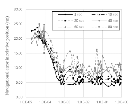
The navigation errors in the y-axis in Fig. 5 are represented by the RMSerr in Eq. (12), which is a root-mean-square (RMS) value of the navigation errors in the relative position at instants when the laser-based measurement was performed throughout the simulation time-period. The navigation error is the difference between the estimated relative orbit and true relative orbit.
In Eq. (12), is the norm of the navigation error at a relative position, which is represented in the RSW frame that originates at the center of the mass of the chief at ki; are the navigation errors of the relative position in the R-, S-, and W-axis of the RSW frame at ki, respectively; and N is the number of instants in which the laser-based measurement is performed, throughout the simulation time-period.
The navigation results are more accurate when α>1×10⁻³ than when α is smaller. Simulations with α≤2×10⁻⁵ could not be implemented, given that the error covariance matrix was not a positive semi-definite at a certain instant, i.e., the matrix was not a true error covariance matrix.
Similar results were obtained in simulation case 2, in which the IOD errors were changed to approximately 200 m and 2 m/s for the relative position and velocity, respectively. The matrices P, Q, and R were determined in the same manner as in simulation case 1. Fig. 6 presents the various navigation errors in the relative position while adjusting α for simulation case 2, and the numbers in the legend in Fig. 6 denote the measurement outage period. In simulation case 2, the navigation results were more accurate when α>1×10⁻³ than when α was smaller.
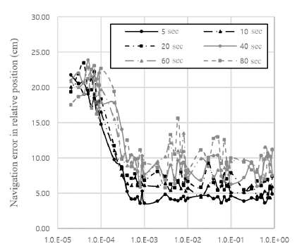
The UKF can accurately estimate the state vector by selecting and propagating sigma points that appropriately correspond to the error covariance of the state vector. However, if α is sufficiently small, only the sigma points that consider nonlinearity and are very close to the mean of the state vector are propagated. This type of propagation is similar to the mean-propagating approach of the EKF, and results in the suboptimal performance of the UKF-based relative navigation. The relative navigation results for α>10-3 are therefore better than those for α<10-3.
The performances of the three relative navigation algorithms based on the EKF, UKF, and LSRF for spacecraft formation flying with intermittent laser-based measurements were compared by implementing relative navigation simulations for simulation cases 1 (small IOD error) and 2 (large IOD error). The scaling parameter α within the UKF-based algorithm was set as 1×10⁻², and the navigation errors in the y-axis in Figs. 7 and 8 were represented by RMSerr in Eq. (12).
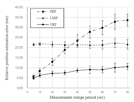
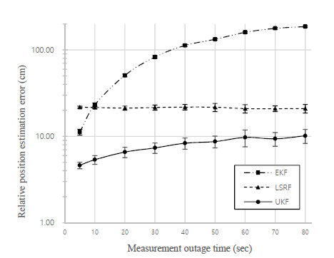
As shown in Figs. 7 and 8, the relative navigation results of the EKF-based algorithm became less accurate as the measurement outage period increased. The results of the UKF-based navigation algorithm also became less accurate as the measurement outage period increased; however, the overall accuracy was improved. Although the navigation errors for the LSRF-based algorithm were larger than those for the EKF- and UKF-based algorithms when the measurement outage period was very small, the error varied within a very small range, even though the measurement outage period increased. In simulation case 1, when the measurement outage periods were increased from 5 sec to 80 sec, the navigation error increased by 493 % for the EKFbased algorithm, 125 % for the UKF-based algorithm, and 0.2 % for the LSRF-based algorithm. The navigation result of the LSRF-based algorithm was 282 % and 361 % less accurate than that of the EKF- and UKF-based algorithms, respectively, when the measurement outage period was 5 sec. The navigation result of the UKF-based algorithm was 69 % and 51 % more accurate than that of the EKF- and LSRFbased algorithms when the measurement outage period was 80 sec. In simulation case 2, when the measurement outage periods were increased from 5 sec to 80 sec, the navigation error increased by 1,577 % for the EKF-based algorithm and 120 % for the UKF-based algorithm. Although the navigation error of the LSRF-based algorithm decreased by 4 %, the standard deviation of the navigation error increased. The navigation result of the LSRF-based algorithm was 94 % and 370 % less accurate than that of the EKF- and UKF-based algorithms, respectively, when the measurement outage period was 5 sec. The navigation result of the UKF-based algorithm was 95 % and 52 % more accurate than that of the EKF- and LSRF-based algorithm when the measurement outage period was 80 sec.
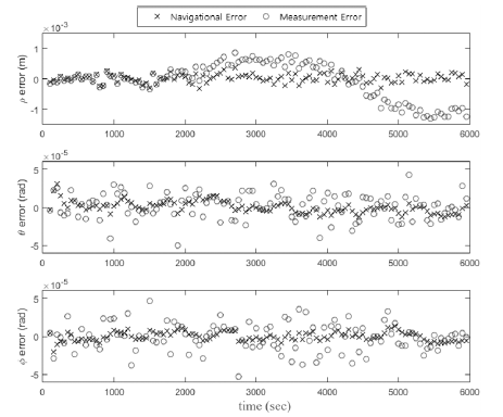
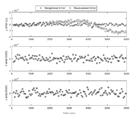
Figs. 9, 10, and 11 present the navigation errors of the EKF-, UKF-, and LSRF-based algorithms, respectively, in the relative position for the spherical frame over the simulation time-period for simulation case 1. The measurement outage period was 50 sec in the figures, and the measurement error in the figures refers to the difference between ρ, θ, and ϕ for the true relative orbit and the laser-based measurement values.
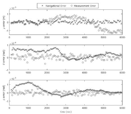
The differences in the navigation performances are due to the characteristics of the filtering algorithms. Based on the assumption that the dynamic and measurement models are quasi-linear, the EKF linearizes dynamic and measurement models in its estimation process (Lee & Alfriend 2007). In addition, the EKF estimates a current state vector based on previously estimated state vectors; thus, errors in previously estimated state vectors continuously accumulate in a currently estimated state vector. In this study, the EKF-based algorithm does not implement measurement correction at a given instant when measurements are not performed. Accordingly, the navigation performance of the EKF-based algorithm decays when the nonlinearity of the system is strengthened by the long measurement outage period (Lee & Alfriend 2003).
However, the UKF does not contain a linearizing approach or assumptions similar to those considered by the EKF. Instead, the UKF selects sigma points that can appropriately capture the mean and error covariance of the state vector that is represented by the GRV, and the sigma points are propagated via the nonlinear dynamic model to precisely predict the state vector and error covariance matrix. Thus, the UKF-based algorithm can estimate the relative orbit more precisely than the EKF-based algorithm.
algorithm. The least squares method estimates the state vector at an instant that minimizes the sum of the square of the measurement residuals. Thus, the navigation and measurement errors in the relative angles (respectively θ and ϕ) are very close, as can be seen in Fig. 11, given that both the laserbased measurement and relative position are represented in the spherical frame. However, the estimated relative distance is closer to the true relative distance than the measured relative distance, given that the scale factor in the measurement model sf eliminates the drift in the measured relative distance. In addition, the estimation performance of the least squares method depends on the quality and quantity of the measurement data. Accordingly, the navigation performance was insensitive to the measurement outage period, given that the same quality and quantity of measurement data were used in the relative navigation, regardless of the measurement outage period. Generally, among the discussed methods, least squares is expected to estimate the state vector with the highest precision, due to its post-processing. However, in this study, only six sets data were used by the LSRF-based algorithm to use the least squares as a real-time estimator. If more measurement data for estimation is inputted to the LSRF-based algorithm, the estimation performance will improve.
The mean computation time for the relative navigation was 0.021 sec for the EKF-based algorithm, 0.082 sec for the UKF-based algorithm, and 1.012 sec for the LSRF-based algorithm. Although the computation times of the EKF- and UKF-based algorithms were similar, the computation time of the LSRF-based algorithm was significantly larger, given that the least squares in the LSRF-based algorithm implemented an iterating differential correction. If 1 sec is a criterion time of real-time relative navigation, the LSRF-based algorithm is not appropriate for real-time relative navigation (Jung et al. 2012).
6 CONCLUSION
In this paper, the EKF-, UKF-, and LSRF-based relative navigations with intermittent laser-based measurements for spacecrafts flying in formation are considered, and the influence of the measurement outage period on the relative navigation performance is presented. Numerical simulations revealed that the relative navigation results of the EKF-based relative navigation algorithm decreased in accuracy as the measurement outage period increased. Considering the significant influence of the scaling parameters (especially α) on the estimation performance of the UKF, the effect of the scaling parameter α on the UKF-based relative navigation was analyzed. The navigation results were more accurate when α>1×10⁻³ than when α was smaller, and α was set as 1×10⁻² when the UKF-based relative navigation algorithm was implemented. The relative navigation results of the UKF-based gorithm also became inaccurate; however, the navigation performance was improved in comparison with that of the EKF-based algorithm. Although the relative navigation results of the LSRF-based algorithm were less accurate than those of the EKF- and UKF-based algorithms when the measurement outage period was very short, the navigation error varied within a very small range, even though the measurement outage period increased. With respect to the relative navigation performance and computation time; among the three algorithms, the UKF-based algorithm is the most appropriate for real-time relative navigation with intermittent laser-based measurements. The results and analyses from this study can be used for the design of relative navigation algorithms for spacecraft formation flying using laser-based measurements. In future studies, the relative navigation performances of the three algorithms under different conditions should be analyzed, especially that of randomly intermittent measurement data.