Journal of Astronomy and Space Sciences

The Korean Space Science Society

2021; 38(2):105-117

pISSN: 2093-5587, eISSN: 2093-1409

DOI: https://doi.org/10.5140/JASS.2021.38.2.105

Research Paper

A Preliminary Impulsive Trajectory Design for (99942) Apophis Rendezvous Mission

Pureum Kim1

, Sang-Young Park1^,†

, Sungki Cho2

, Jung Hyun Jo2

¹Astrodynamics and Control Lab., Department of Astronomy, Yonsei University, Seoul 03722, Korea

²Korea Astronomy and Space Science Institute, Daejeon 34055, Korea

^†Corresponding Author Tel: +82-2-2123-5687, E-mail: spark624@yonsei.ac.kr

© The Korean Space Science Society. All rights reserved. This is an Open-Access article distributed under the terms of the Creative Commons Attribution Non-Commercial License (http://creativecommons.org/licenses/by-nc/3.0/) which permits unrestricted non-commercial use, distribution, and reproduction in any medium, provided the original work is properly cited.

Received: Jan 27, 2021; Revised: May 14, 2021; Accepted: May 17, 2021

Abstract

In this study, a preliminary trajectory design is conducted for a conceptual spacecraft mission to a near-Earth asteroid (NEA) (99942) Apophis, which is expected to pass by Earth merely 32,000 km from the Earth’s surface in 2029. This close approach event will provide us with a unique opportunity to study changes induced in asteroids during close approaches to massive bodies, as well as the general properties of NEAs. The conceptual mission is set to arrive at and rendezvous with Apophis in 2028 for an advanced study of the asteroid, and some near-optimal (in terms of fuel consumption) trajectories under this mission architecture are to be investigated using a global optimization algorithm called monotonic basin hopping. It is shown that trajectories with a single swing-by from Venus or Earth, or even simpler ones without gravity assist, are the most feasible. In addition, launch opportunities in 2029 yield another possible strategy of leaving Earth around the 2029 close approach event and simply following the asteroid thereafter, which may be an alternative fuel-efficient option that can be adopted if advanced studies of Apophis are not required.

Keywords: trajectory design; impulsive trajectory; asteroid exploration; (99942) Apophis; monotonic basin hopping

1. INTRODUCTION

There is an increasing demand for exploration missions to near-Earth asteroids (NEA), as evidenced by several recently conducted missions such as Hayabusa (Kawaguchi et al. 2008), Hayabusa2 (Watanabe et al. 2017), and OSIRISREx (Lauretta et al. 2017), as well as planned missions such as DESTINY+ (Sarli et al. 2018) and ZhengHe (Jin et al. 2020), both of which have planned launch dates in the mid- 2020s. The increasing demand stems from several aspects of asteroid exploration that cannot be fully accomplished with traditionally favored planetary exploration missions. For planetary scientists, understanding these small rocky or icy bodies can provide them with new clues on how the solar system has evolved, as they are pristine remnants of the tumultuous early solar system. NEA exploration is also anticipated to have commercial value within a few decades owing to the abundance of rare elements on Earth and their relative ease of access (Andrews et al. 2015).

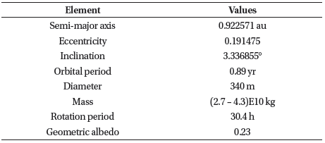
At the same time, NEAs can pose a huge threat to humankind in the form of impact events. Asteroid (99942) Apophis (originally designated 2004 MN4) is a well-known NEA that was once computed to have a high probability of hitting Earth in 2029. Although the possibility of this 400-m-wide asteroid impacting Earth in 2029 has since been ruled out following precise orbit determination with extensive observations, the asteroid is still expected to approach Earth at a distance closer than geosynchronous satellites on April 13, 2029 (Brozović et al. 2018). This approach is expected to bring about several physical and geological changes to Apophis, including changes in spin state and surface morphology (Yu et al. 2014;Souchay et al. 2018;DeMartini et al. 2019); accordingly, the 2029 approach of Apophis will present a unique opportunity to study the effect of seismic events on small asteroids following a close planetary flyby, as well as the opportunity to deepen our general understanding of small bodies that may threaten humanity in the future, making Apophis an attractive target for near-future NEA exploration missions. Table 1 lists some orbital and physical information on Apophis. Please note that the orbital parameters listed in the table are those of the epoch May 31, 2020. As Apophis makes close encounters with Earth several times in the future, its orbital elements will undergo a significant change with each encounter.

Table 1. Some selected orbital and physical parameters of Apophis (epoch May 31, 2020). The data were retrieved from the JPL Small-Body Database Browser

Download Excel Table

Trajectory optimization assumes a crucial role in designing interplanetary missions as the trajectory is intimately connected to the mission cost and feasibility, and missions to NEAs are no exception. Global optimization algorithms are considered an efficient modern approach to spacetrajectory optimization problems. Global optimization algorithms often employ heuristic strategies to investigate the given search space efficiently and search for good solutions that are scattered around. The concept of adopting them for interplanetary trajectory design was once considered inefficient when the idea was first presented in the 1990s (Rauwolf & Coverstone-Carroll 1996;Hartmann et al. 1998), but with ever-increasing computing speed, the approach soon became recognized as a practical way of designing interplanetary trajectories. The monotonic basin hopping (MBH) algorithm (Wales & Doye 1997) used in this study as the main optimization algorithm is one such global optimization algorithm. The MBH algorithm relies on the successive use of a local search algorithm to reach the global optimum, and has shown advantages over other widely known global optimization algorithms in the area of space trajectory problems (Vasile et al. 2010;Kim 2019).

Depending on the type of spacecraft propulsion, interplanetary trajectories can be classified as continuous low-thrust and impulsive high-thrust trajectories. Although interplanetary missions employing low-thrust engines are gaining popularity, high-thrust engines are also favored, as shown by past and upcoming missions such as NEAR Shoemaker (Prockter et al. 2002), Rosetta (Glassmeier et al. 2007), OSIRIS-REx (Williams et al. 2018), and Lucy (Englander et al. 2019). These two different types of trajectories usually require completely different optimization strategies, but the global optimization approach can be applied to optimize both of them (Vasile et al. 2010;Englander & Conway 2017). In the current study, we focus on the design of impulsive trajectories, which can be considered as an idealized version of high-thrust trajectories. To further simplify the problem, impulsive trajectories will be designed under the assumption of a zerosphere of influence patched conic approximation (Vasile & De Pascale 2006). These two simplifications allow for the rapid optimization of preliminary trajectories without sacrificing too much integrity. The resulting preliminary trajectories can then be used as a stepping stone toward the design of more elaborate high-thrust trajectories that also fully account for the complex dynamics of the solar system. When designing interplanetary trajectories, deep space maneuvers (DSMs) and gravity assists (also called swing-by’s) are often included to reduce the amount of fuel consumption. However, at the same time, they provide additional complexity in the preliminary trajectory design process because the number, order, and exact timing of these fuel-saving techniques have a critical impact on the amount of fuel required for the journey. Global optimization algorithms with appropriate optimization problem transcription can be quite powerful when optimizing such complex trajectories.

In this paper, the preliminary design of impulsive trajectories to Apophis is discussed with the purpose of making a rendezvous with the asteroid in 2028-2029. Although there have been a few studies on preliminary mission or trajectory design for future Apophis missions, some were designed under the assumption of an Apophis deflection mission (Dachwald & Wie 2007;Li et al. 2014), while others were given as examples of novel trajectory design approaches (Schutze et al. 2011;Gong et al. 2015). An extensive trajectory design analysis for Apophis missions under several different mission architectures was conducted by Wagner and Wie (2013), but the analysis was limited to two-impulse ballistic trajectories only. However, the preliminary mission analysis performed in this study has a specific scientific goal of exploring Apophis during the close-approach event of 2029. Furthermore, trajectories involving flybys and DSMs were also explored in this study, enabling the discovery of possibly more efficient trajectories than simple ballistic trajectories. It is anticipated that this research can be used as a reference for performing a cost-benefit analysis or establishing a baseline for future exploration missions in the future. For instance, the launch/ rendezvous window analysis presented here can be used to analyze and select several possible launch/rendezvous date options that can satisfy other mission constraints, as the most fuel-efficient trajectory may not be the best choice when other factors (such as journey duration or amount of time allotted for Apophis pre-study) are taken into account.

The remainder of this paper is organized as follows. As with all solving processes of optimization problems, the problem and cost function need to be clearly defined first, and then an adequate optimization method needs to be chosen and applied to the problem. Section 2 presents the precise definition of the cost function to be minimized, and a few different types of impulsive trajectory problems investigated herein are discussed in detail. Section 3 is devoted to the concise introduction of the MBH algorithm used to locate near-optimal solutions to the problems. The entire design procedure and results, along with some of the near-optimal sample trajectories, are presented in Section 4. The first two subsections of Section 4 focus on trajectories where the journey ends in 2028, so the spacecraft will have a few months to study Apophis before the eventual close approach. The third subsection discusses the ballistic trajectory scenario in which the entire journey is covered within the year 2029. Conclusions and possible future work are summarized in Section 5.

2. PROBLEM FORMULATION

Fundamentally, trajectory optimization problems constitute an optimal control problem. However, for them to be solved with common global optimization algorithms, they need to be transcribed into finite-dimensional nonlinear programming (NLP) problems. During the problem transcription procedure, the sophisticated dynamic constraints acting on the spacecraft are simplified. In addition, solution trajectories are assumed to consist of a predetermined sequence of maneuvers, and several different NLP problems can be formed depending on the maneuvers used and their exact number and order. The most frequently used simplified dynamics is the zero-sphere of influence patched conic approximation (also called the linked-conic approximation). Under this approximation, a spacecraft trajectory is simply reduced to several arcs of heliocentric two-body orbits connected together; points connecting two different arcs represent the locations at which maneuvers are used. In addition, all maneuvers related to the gravity of planetary bodies, such as departure, arrival, and gravity assists are assumed to occur instantaneously at the center of the celestial body. In other words, the radii of the spheres of influence of all planetary bodies are assumed to be zero. This approximation allows for a very rapid generation of interplanetary trajectories without an initial guess, and it is thus often adopted in preliminary trajectory design (Vasile & De Pascale 2006;Yam et al. 2009).

In the following subsections, three different types of impulsive trajectory transcriptions are introduced: ballistic trajectory, one deep space maneuver (1DSM) trajectory, and multiple gravity assists with one deep space maneuver per leg (MGA-1DSM) trajectory. The three trajectory models involve different maneuvering sequences, but they all assume a linked-conic approximation. From now on, part of the trajectory that connects one planetary body to another is referred to as a leg. A leg is comprised of one or more segments, which are basically heliocentric Lambert arcs, and segments in one leg are connected by DSMs. Each segment is denoted in the form of LlSs, where lowercase l and s refer to the leg number and segment number, respectively. For instance, L3S2 refers to the second segment of the third leg.

2.1 Cost Function

In this study, the cost function is defined as the total delta-v that is required to complete the trajectory from escaping the Earth parking orbit to making a rendezvous with Apophis. It is assumed that the spacecraft departs from a circular low-Earth parking orbit at an altitude of 600 km. The delta-v required for leaving the parking orbit to be inserted into a heliocentric interplanetary trajectory can be computed using Eq. (1)

Δ v 0 = ‖ v ∞, 0 ‖ 2 + 2 μ E r E + h − μ E r E + h

(1)

where μ_E, r_E, and h represent the standard gravitational parameter of the Earth, Earth radius, and parking orbit altitude, respectively. The hyperbolic excess velocity vector (also called the v-infinity vector) associated with leaving Earth, $υ ∞, 0$ , is defined as the difference between the Earth’s velocity vector and the spacecraft’s velocity vector (after the first impulsive maneuver is acted upon by the spacecraft) in the J2000 heliocentric ecliptic frame (refer to Fig. 1 for an example). It should be noted that owing to the nonlinearity of Eq. (1), the use of different parking orbit altitudes can lead to different optimal trajectories.

Fig. 1. Simplified illustration of a ballistic trajectory. Planetary orbits and heliocentric spacecraft trajectory are represented by thin black lines and thick gray lines, respectively. Each heliocentric arc making up the trajectory is labeled with its leg number (following L) and segment number (following S).

Download Original Figure

As Apophis is not large enough to exert a meaningful gravitational pull, it is reasonable to assume that the delta-v that is required to rendezvous with it is the same as the magnitude of the hyperbolic excess velocity vector at arriving Apophis, $υ ∞, f$ , as in Eq. (2). The hyperbolic excess velocity $υ ∞, f$ is defined as the difference between Apophis’s velocity vector and the spacecraft’s velocity vector (before the last impulsive maneuver is exerted) in the heliocentric ecliptic frame (refer to Fig. 1 for an example).

Δ υ f = ‖ υ ∞, f ‖

(2)

Then, the cost function is the sum of Eqs. (1)–(2) along with delta-v values for all of the DSMs used, as given by Eq. (3).

J (X) = Σ Δ υ = Δ υ 0 + Δ υ f + Σ Δ υ D S M

(3)

In the equation, X denotes a decision vector, composed of parameters to be optimized to minimize the cost function. The length and composition of the decision vector are different for each trajectory model, and detailed information for each model is discussed in the following subsections.

2.2 Ballistic Trajectory

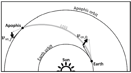
A ballistic trajectory is the simplest possible interplanetary trajectory. For ballistic rendezvous missions, only two impulsive maneuvers are required: one to escape Earth and the other to rendezvous with the target body. Without any other maneuver in between them, the trajectory is simply a single heliocentric two-body arc connecting the Earth and the target body. In other words, a ballistic trajectory consists of a single leg, which also contains only one segment. An example of a ballistic trajectory is shown in Fig. 1.

When the initial time (time on leaving Earth) t₀ and the final time (time on arrival at the target body) t_f are specified, the position and velocity of Earth and Apophis at those times can be computed from celestial ephemerides. DE430 (Folkner et al. 2014) was used as a planetary ephemeris, and the Apophis ephemeris was obtained from NASA JPL Horizons (n.d.). An open-source geometry system for space science missions called SPICE (Acton et al. 2018) was used to process the ephemeris data. With the two end positions now known, the two-body arc linking the two positions with a time duration of T = T_L₁ = T_L1S1 = t_f – t₀ can be computed by solving Lambert’s problem. A robust Lambert solver proposed by Oldenhuis (2020), which hybridized two solvers by Izzo (2015) and Gooding (1990), was used. It should be noted that although Lambert’s problem usually has more than one solution, we chose to use only the counter-clockwise zero-revolution solution; with this restriction there can be no more than one solution for any Lambert’s problem. Now that the trajectory is determined, the two excess velocity vectors $υ ∞, 0$ and $υ ∞, f$ can be easily obtained by simply computing the differences between the heliocentric velocity vectors of the spacecraft and the two celestial bodies at initial and final time.

From the two excess velocity vectors, the required deltav’s Δυ₀ and Δυ_f can be computed using Eqs. (1)–(2), and the cost function for ballistic trajectories is simply the sum of the two delta-v values, as ballistic trajectories do not use DSMs. The decision vector X for ballistic trajectories is a two-dimensional vector given by Eq. (4).

X ≡ [t 0 t f]

(4)

2.3 1DSM Trajectory

A 1DSM trajectory allows a single DSM during the entire trip, and this additional DSM can sometimes lead to a decrease in fuel usage compared to simple ballistic trajectories. A 1DSM trajectory is made up of two different heliocentric arcs connected by a DSM, and it can therefore be considered to consist of one leg that is comprised of two segments. An example of the 1DSM trajectory is shown in Fig. 2. Although it is possible to add more DSMs in between to form nDSM trajectories, they make the optimization problem complex because each additional DSM introduces four additional degrees of freedom to the NLP problem. However, these additional DSMs rarely yield a meaningful decrease in total delta-v usage (Kim 2019). For this reason, the nDSM trajectories were not discussed in this study.

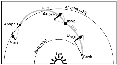
Fig. 2. Simplified illustration of a 1DSM trajectory. Planetary orbits and heliocentric spacecraft trajectory are represented by thin black lines and thick gray lines, respectively. Each heliocentric arc making up the trajectory is labeled with its leg number (following L) and segment number (following S). DSM, deep space maneuvers.

Download Original Figure

To define 1DSM trajectories, six parameters are required: three time-related parameters and three parameters for defining the v-infinity vector $υ ∞, 0$ on leaving Earth. The three time-related parameters are the initial time t₀, final time t_f, and time proportion parameter 0 < η_L1S1 < 1. The entire trip duration T = T_L₁ and trip duration for each segment, which are denoted by T_L1S1 and T_L1S2, are simply computed by Eq. (5).

T = T L 1 = t f − t 0 T L 1 S 1 = T L 1 η L 1 S 1, T L 1 S 2 = T L 1 (1 − η L 1 S 1)

(5)

In 1DSM trajectories, unlike ballistic trajectories, $υ ∞, 0$ is not obtained by comparing the Lambert solution and Earth’s velocity vector at t₀, but it is defined by three optimization parameters: its magnitude $υ ∞, 0$ and its direction represented by ecliptic longitude $l ∞, 0$ and ecliptic latitude b_∞,0. With these three parameters, $υ ∞, 0$ can be easily formed, and the heliocentric velocity vector $v 0 +$ of the spacecraft leaving Earth is described by Eq. (6), where $v 0 −$ denotes the heliocentric velocity of the Earth at t₀.

v 0 + = v 0 − + v ∞, 0 = v 0 − + v ∞, 0 [cos (b ∞, 0) cos (I ∞, 0) cos (b ∞, 0) sin (I ∞, 0) sin (b ∞, 0)]

(6)

The first segment (L1S1) is obtained via the two-body propagation of the spacecraft’s state vector for the duration of T_L1S1, as the other end of the arc is unknown. In contrast, the second segment (L1S2) should be connected by solving Lambert’s problem as the positions of both ends are known, and $υ ∞, f$ can be computed by taking the difference between this Lambert solution and the Apophis velocity vector at t_f.

The amount of delta-v required for the DSM, Δυ_DSM₁, can be easily computed as the incoming velocity (final velocity of L1S1) and outgoing velocity (initial velocity of L1S2) can be easily obtained. The total delta-v for the 1DSM trajectories is the summation of Δυ₀, Δυ_f, and Δυ_DSM₁, as shown in Eq. (3), where Δυ₀ and Δυ_f can be obtained from Eqs. (1)–(2). The decision vector X for the 1DSM trajectories is a six-dimensional vector given by Eq. (7).

X ≡ [t 0 t f η L 1 S 1 υ ∞, 0 l ∞, 0 b ∞, 0]

(7)

2.4 MGA-1DSM Trajectory

The MGA-1DSM model by Vasile & De Pascale (2006) is distinguished from the previous two models in that it allows one or more gravity assists. MGA-1DSM trajectories can consist of any number of gravity assists, and one DSM is required for each leg. In other words, an MGA-1DSM trajectory with n gravity assists consists of n + 1 legs, each of which is made up of two segments. An example of the MGA-1DSM trajectory with two gravity assists is shown in Fig. 3. Similar to the case of nDSM trajectories, MGAnDSM transcription, where more than one DSM is allowed per leg, is possible, but it is impractical in terms of the cost effectiveness of the optimization process (Vavrina et al. 2016).

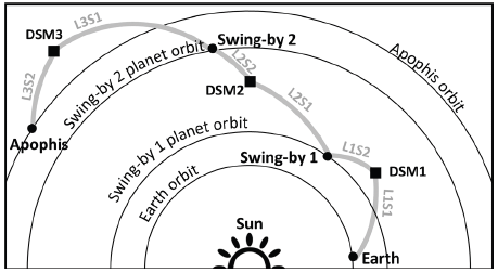
Fig. 3. Simplified illustration of an MGA-1DSM trajectory with two gravity assists. Planetary orbits and heliocentric spacecraft trajectory are represented by thin black lines and thick gray lines, respectively. Each heliocentric arc making up the trajectory is labeled with its leg number (following L) and segment number (following S). Delta-v vectors are not explicitly shown for the sake of simplicity. DSM, deep space maneuvers. MGA-1DSM, multiple gravity assists with one deep space maneuver per leg.

Download Original Figure

To define an MGA-1DSM trajectory with n gravity assists, a total of 4n + 6 decision variables are required. Among them, 2n + 3 variables are time-related variables that are needed to define the initial time and final time, as well as the time duration for each segment. For instance, an MGA- 1DSM trajectory with two gravity assists requires seven time-related parameters. From these parameters, the total trip duration T, duration for each leg T_L₁, and duration for each segment T_LlSs can be computed as in Eq. (8).

T = t f − t 0 T L 1 = T η L 1, T L 2 = T (1 − η L 1), T L 3 = T (1 − η L 1) (1 − η L 2) T L l S 1 = T L l η L l S 1, T L l S 2 = T L 1 (1 − η L l S 1) for l = 1, 2, 3

(8)

Three parameters are still required to define $υ ∞, 0$ , as is the case with a 1DSM trajectory. Here, the number of parameters (three) is independent of the number of swingby’s, as these parameters are used to describe the departure maneuver from Earth. The remaining 2n parameters are used to define the gravity assists. At the end of each leg (except for the last leg), a planetary swing-by is assumed to occur instantaneously. To define each gravity assist, two parameters (the minimum distance R to the swing-by planet and B-plane angle θ) are required to compute the velocity vector difference before and after the gravity assist (Kawakatsu 2009), requiring 2n parameters to cover all gravity assists.

The delta-v values required to leave Earth (Δυ₀) and to rendezvous with Apophis (Δυ_f) can again be obtained using Eqs. (1)–(2), and the delta-v for each DSM (Δυ_DSM₁, Δυ_DSM₂, ..., Δυ_DSM_(n+1)) can be computed from the difference between the incoming and outgoing velocities at each DSM location. The cost function for the MGA-1DSM trajectories is given by Eq. (3), where the number of DSMs is n + 1.

As an example, the decision vector for the MGA-1DSM trajectories with two gravity assists (consisting of 14 parameters) is presented in Eq. (9). The decision vector can be easily modified for a different number of gravity assists by adding (or removing) time and gravity assist parameters. It should be noted that the decision vector itself does not have information about the swing-by planet, and thus the gravity assist planet sequence should be decided in advance to define a unique trajectory. With these 4n + 6 parameters and the known swing-by sequence, an MGA- 1DSM trajectory can be uniquely defined by solving for each segment with two-body propagation (first segment for each leg) and Lambert’s problem (second segment for each leg).

X ≡ [t 0 t f η L 1 η L 2 η L 1 S 1 η L 2 S 1 η L 3 S 1 v ∞, 0 l ∞, 0 b ∞, 0 R 1 R 2 θ 1 θ 2]

(9)

3. MONOTONIC BASIN HOPPING ALGORITHM

The MBH algorithm is a global optimization algorithm that uses a local search algorithm successively to approach the globally optimal solution. It was originally developed by chemists Wales and Doye (1997) to discover molecular structures with the lowest energy. While there is no optimization algorithm that is superior to other algorithms for all kinds of problems, some may be better suited than others for specific problems. In the case of interplanetary trajectory optimization, MBH has been proven to outperform other well-known algorithms, such as genetic algorithms (GAs), particle swarm optimization (PSO), and multi-start (MS) (Vasile et al. 2010;Kim 2019). According to Addis et al. (2011), the superior performance of MBH in the realm of space trajectory optimization problems may hint at the possible funnel structure of these problems.

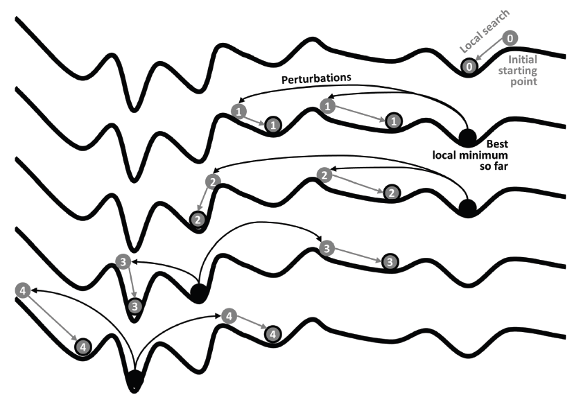
The MBH algorithm attempts to find the global optimal solution inside a given search space by locating a large number of local optimal solutions. As the number of visited local optima increases, the likelihood grows that there exists the global optimum among them. From this viewpoint, the algorithm is similar to the MS algorithm, which is also a local search-based algorithm. In the MS algorithm, a number of starting points are randomly selected inside the feasible region, and local searches are run from each point (Martí et al. 2018). Each local search will arrive at a local minimum, and the best local minimum among them is chosen as the solution of the algorithm. In the MBH algorithm, a single starting point is randomly chosen, and thereafter, the corresponding local minimum is determined by the local search algorithm. Then, another random starting point (called a perturbed point) is generated in the neighborhood of the best minimum known so far, and then the local search algorithm is run from the perturbed point to find the corresponding local minimum. If the newly found local optimum is better than the best one that is known until then, it replaces its position as the best-known minimum. This process is repeated until a stopping condition (such as the number of successive failures in finding a better local minimum) is satisfied. In theory, MS attempts to locate the global minimum by scanning the entire search space, whereas MBH starts from a random local minimum and attempts to reach the global minimum by continually hopping to a lower basin nearby (hence the name).

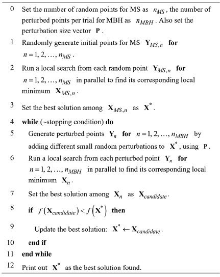
To further enhance the performance of MBH, a parallelized version of MBH presented by McCarty and McGuire (2018) was utilized in this study. In this variant of MBH, several perturbed points are generated simultaneously in one step, and local searches are run from each point in parallel. Then, the best among the newly found local minima is compared with the current best minimum. Fig. 4 schematically shows the procedure of this parallel variant of MBH, where two perturbed points are generated in one step. In Fig. 5, a simplified pseudocode for the parallel MBH algorithm is presented. As can be seen in the pseudocode, the MBH algorithm used in this study also takes advantage of the MS algorithm when generating a good initial starting point for MBH. For this research, n_MS and n_MBH were chosen as 64 and 32, respectively. The perturbation size vector P was chosen such that the perturbation size for each variable was 5% of the bound size.

Fig. 4. Schematic procedure of parallelized MBH algorithm. In this example, it is assumed that two perturbed points are generated in one step. MBH, monotonic basin hopping.

Download Original Figure

Fig. 5. Simplified pseudocode for the parallel MBH algorithm. MBH, monotonic basin hopping.

Download Original Figure

4. RESULTS

This section discusses preliminary trajectory design procedures used in this study, and an analysis of the results is presented. Some near-optimal trajectories for a future Apophis exploration mission are also shown as examples. The first two subsections discuss the scenario where the spacecraft makes a rendezvous with Apophis in the year 2028, which will give the spacecraft several months for the advance exploration of Apophis before the Apophis – Earth close approach event in April 2029. The first subsection focuses on the identification of a few feasible maneuver/ swing-by sequences, and in the second subsection, the chosen sequences are analyzed in more detail. In the third subsection, a different scenario is discussed, where the entire trip from Earth to Apophis will occur in 2029 with the spacecraft following a simple ballistic trajectory. While this scenario may not allow the advanced study of the asteroid before the close approach event, it may be considered as a viable option if there is no need for an early visit (for instance, if pre-approach observation can be adequately performed via ground- or space-based telescopes). As discussed later in detail, this scenario has some advantages, such as a lower total delta-v and shorter journey.

4.1 Feasible Sequence Identification

To increase the efficiency of the trajectory design process, it is preferable to identify a few feasible maneuver/swingby sequences before in-depth analyses are performed. For the MGA-1DSM model, several swing-by sequences were manually chosen to be tested for feasibility. As the pre- 2029 nominal heliocentric orbit of Apophis lies between the orbits of Venus and Mars, Venus, Earth, and Mars were chosen as candidate swing-by planets, and the number of gravity assists was limited to two; thus, the number of possible MGA-1DSM sequences is 12. In total, 14 sequences (three with a single gravity assist, nine with two assists, and two without any assists) were chosen as candidates for this feasibility analysis. From now on, MGA-1DSM sequences are denoted by abbreviations of the visiting order; for instance, the EVMA sequence indicates that it is an MGA- 1DSM sequence with two gravity assists that begins from Earth and performs two swing-by’s at Venus and then Mars, and then reaches Apophis in the end.

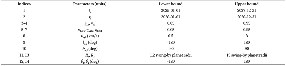
For each of the 14 candidate sequences, the parallel MBH algorithm was run 50 times with different optimization time limits depending on the dimension of the optimization problem. All computations were performed on a PC with an Intel Core i9-7960X (16 cores). The bounds of the parameters used in this study are listed in Table 2. The indices listed in the table were assigned under the assumption of the MGA- 1DSM problem with two gravity assists, so they can be different for the rest of the problems. Note that the range for angular parameters such as $l ∞, 0$ , b_∞,0, and θ were set to be wider than those listed in the table for the local optimization algorithm. This was done to prevent the numerical pitfall of the local optimal solution from becoming stuck at one boundary when it can actually proceed beyond that boundary (Kim 2019).

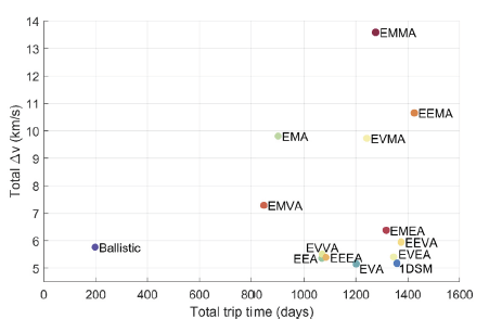
Table 2. Parameter bounds used for feasible sequence identification

Download Excel Table

In Fig. 6, the best solution for each maneuver sequence is plotted in the total trip time – total delta-v plot. Here, the best solution is simply defined as the solution with the lowest cost function value (that is, the one with the lowest total delta-v value, as defined in Eq. (3)) among the 50 solutions obtained. It should be noted that the total trip time given in the figure is that of the fuel-optimal solution, and is not representative of that sequence itself. As will be shown in the next subsection, a shorter trip than that shown in Fig. 6 is possible by allowing a slightly larger fuel consumption. From the figure, we concluded that the 1DSM, EVA, and EEA sequences are the most feasible sequences among the 14 candidate sequences. The minimum total delta-v usage for these sequences was found to be 5.180, 5.164, and 5.365 km/s, respectively. Although some sequences involving two gravity assists, namely EVVA, EVEA, and EEEA, also displayed delta-v usage that had similar orders of magnitude, we excluded them from the thorough analyses because the additional gravity assist did not appear to aid in reducing fuel consumption, but it instead only made the trip longer and more complex.

Fig. 6. Comparison of the most optimal solution of each sequence in the total trip time vs. total delta-v graph, where the optimal solution is defined as requiring the least total delta-v. MGA-1DSM sequences are denoted by abbreviations of the visiting order; for instance, EVMA stands for Earth-Venus- Mars-Apophis.

Download Original Figure

4.2 Detailed Analyses on Feasible Sequences

More thorough analyses with respect to departure and arrival times were conducted for the three sequences that were identified as feasible in Subsection 4.1. Bounds for the initial time t₀ and final time t_f (listed in Table 2) were split into small blocks so that each time block covered one month of t₀ and one month of t_f. Except for the bounds of the initial and final times, all of the other parameter bounds remained unchanged. For the EVA and EEA sequences, time blocks that correspond to the total trip time of one year or less were excluded from the analyses, as such a short trip for those two sequences was deemed infeasible. For each time block, the MBH algorithm was run 20 times, and the most optimal solution (which again is the result with the least total delta-v) was identified and selected as the best trajectory for that time block.

Fig. 7 shows the variation in the total delta-v value with respect to the departure and arrival times. For all three sequences, an obvious trend is that the fuel usage is heavily dependent on when the spacecraft departs from Earth, but it is much less affected by the time that it reaches and makes its rendezvous with Apophis. For the EVA sequence, the opportunities for near-optimal trajectories that require delta-v values of less than 5.5 km/s exist only until early 2025. However, for the other two sequences, such nearoptimal opportunities persist until 2027, even though these trajectories require the spacecraft to reach Apophis in late 2028. A few such good occasions were manually identified, and are represented as yellow diamonds in the figure. More detailed information on these example trajectories is listed in Table 3, and four cases among them that have a total trip time of 700 days or fewer are visualized in Fig. 8. In the table, the characteristic energy (C₃) is simply equal to $‖ υ ∞, 0 ‖ 2$ . The last column of the table is the declination δ_∞,0 of v-infinity vectors on leaving Earth ( $υ ∞, 0$ ). It is defined in the same way as the ecliptic latitude b_∞,0 of v-infinity vectors, except that the declination should be measured in the Earth equatorial coordinates instead of ecliptic coordinates. These v-infinity declination values place limit on the allowed range of the Earth parking orbit inclination i_p of the spacecraft, as in Eq. (10).

Fig. 7. Minimum total delta-v required for the three feasible sequences, for different Earth departure and Apophis arrival dates. (a) 1DSM trajectories, (b) EVA trajectories, (c) EEA trajectories. Yellow diamonds represent selected trajectories that require total delta-v values of less than 5.5 km/s. Refer to Table 3 for more information on the selected trajectories. DSM, deep space maneuvers; EVA, Earth- Venus-Apophis; EEA, Earth-Earth-Apophis.

Download Original Figure

Table 3. Detailed information on example trajectories

Download Excel Table

Fig. 8. Trajectories for four selected example cases. (a) Case 3, (b) Case 4, (c) Case 8, and (d) Case 10. Spacecraft trajectories are represented by thick black lines. Thin blue and red lines represent heliocentric orbits of Earth and Apophis (before being deflected by Earth’s gravity), respectively. Information about impulsive maneuvers (except for DSMs that are less than 0.001 km/s) is shown on tooltips. DSM, deep space maneuvers.

Download Original Figure

| δ ∞, 0 | ≤ i p ≤ 180 o − | δ ∞, 0 |

(10)

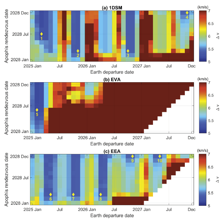
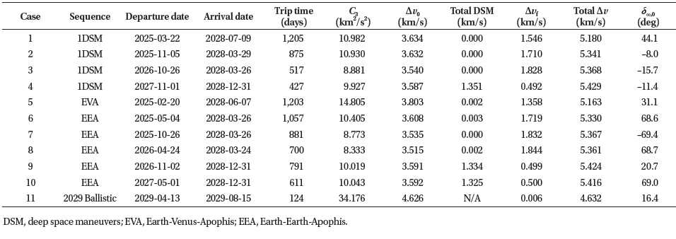
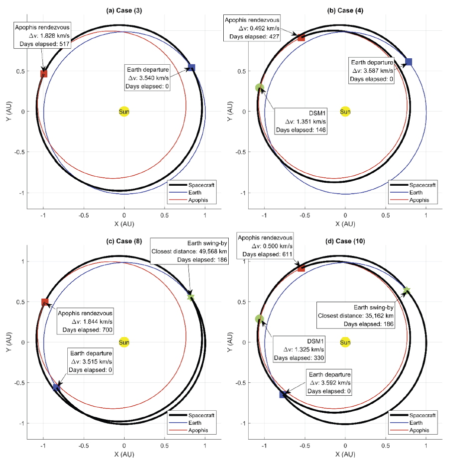
It can be seen from Table 3 that Cases 1–3 of the 1DSM trajectories require almost zero-magnitude DSM, making them basically ballistic trajectories. They correspond to multi-revolution solutions of Lambert’s problem, as can be seen in the trajectory of Case 3 in Fig. 8(a). These multirevolution ballistic trajectories were not found during the ballistic trajectory optimization in Subsection 4.1 because we opted to use only the zero-revolution solution of Lambert’s problem, as mentioned in Subsection 2.2. However, because of the formation of the 1DSM model, such multi-revolution ballistic trajectories can be found during the optimization of 1DSM trajectories in the form of trajectories with a nearly zero magnitude DSM.

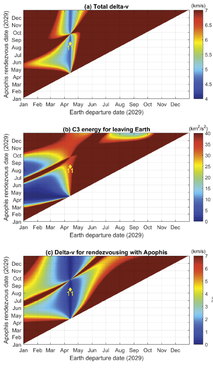
4.3 Ballistic Rendezvous Opportunities in 2029

Depending on the specific scientific goal of the conceptual mission, it may be unnecessary to rendezvous with Apophis earlier than the close-approach event. For such a mission, one can consider adopting a simple ballistic trajectory where both the Earth departure and Apophis rendezvous occur in 2029. 1DSM trajectories can also be adopted, but they do not offer a meaningful advantage over ballistic trajectories in this case, and thus are not discussed herein. In Fig. 9, the total delta-v, C₃ energy, and delta-v for Apophis rendezvous for 2029 ballistic trajectories are plotted as a pork-chop plot. It was assumed that ballistic trajectories require at least three days of trip time. It is very evident that there is a specific departure time that ensures low total delta-v usage at around 4.63 km/s, and as long as the departure time is fixed at that time, the rendezvous time is of minute importance in terms of fuel consumption. The specific optimal departure date is April 13, which coincides with the Apophis close-approach event. One example solution where the spacecraft leaves Earth on April 13 and rendezvouses with Apophis on August 15 is represented as the yellow diamond (11) in Fig. 9, and more detailed information is given in Table 3 as Case 11. As can be inferred from the departure date and very low delta-v required to rendezvous, this trajectory (and all the other trajectories sharing the same departure time) corresponds to the case where the spacecraft virtually accompanies Apophis through its journey along its newly deflected heliocentric orbit.

Fig. 9. Analyses of 2029 ballistic trajectories, for different Earth departure date and Apophis rendezvous date. (a) Total delta-v required, (b) C₃ energy required to leave Earth, (c) Delta-v required to rendezvous with Apophis. Each tick refers to the beginning of each month. Yellow diamond represents a selected example trajectory; refer to Table 3 for more information on this trajectory.

Download Original Figure

5. CONCLUSIONS

In this study, preliminary trajectory design and analyses for a future mission to visit and inspect asteroid (99942) Apophis around its 2029 close approach to Earth were performed under the assumption of using impulsive maneuvers. Several different types of trajectories that may or may not include gravity assists were analyzed, and relatively simple trajectories, such as multi-revolution ballistic trajectories, 1DSM trajectories, and MGA-1DSM trajectories with a single gravity assist from Earth or Venus, were found to be the most feasible. For the spacecraft to rendezvous with Apophis before the end of 2028, the latest departure opportunity requiring a delta-v that is less than 5.5 km/s is in November 2027. It was also found that in the event that it is not necessary to arrive at Apophis before the close approach event, the strategy of letting the spacecraft accompany Apophis along its deflected orbit immediately after the close approach event may require an even less total delta-v of approximately 4.6 km/s.

The preliminary analyses in this study were conducted under the assumption that the spacecraft leaves from a 600- km altitude Earth parking orbit, and the cost function was defined simply as the total delta-v required to depart from the parking orbit until the rendezvous. It should be noted that the result itself will change under a different departure scenario (such as a change in the altitude of the parking orbit or the use of a launch vehicle from Earth), but the general procedure of the preliminary design used in this study can still be followed. Starting from the preliminary design obtained through this procedure, high-fidelity trajectories can be built and fine-tuned. Such high-fidelity trajectories should reflect both complex dynamics and more realistic constraints, and are likely to require more maneuvers than those used in the preliminary trajectory.

ACKNOWLEDGMENTS

This research was supported by the Korea Astronomy and Space Science Institute under the R&D program (Project No. 2021-1-854-05) supervised by the Ministry of Science and ICT.

Notes

Pureum Kim https://orcid.org/0000-0001-9922-9814

Sang-Young Park https://orcid.org/0000-0002-1962-4038

Sungki Cho https://orcid.org/0000-0003-4538-7571

Jung Hyun Jo https://orcid.org/0000-0003-1906-8075

References

Acton C, Bachman N, Semenov B, Wright E, A look towards the future in the handling of space science mission geometry, Planet. Space Sci. 150, 9-12 (2018).

Addis B, Cassioli A, Locatelli M, Schoen F, A global optimization method for the design of space trajectories, Comput. Optim. Appl. 48, 635-652 (2011).

Andrews DG, Bonner KD, Butterworth AW, Calvert HR, Dagang BRH, et al., Defining a successful commercial asteroid mining program, Acta Astronaut. 108, 106-118 (2015).

Brozović M, Benner LAM, McMichael JG, Giorgini JD, Pravec P, et al., Goldstone and Arecibo radar observations of (99942) Apophis in 2012–2013, Icarus. 300, 115-128 (2018).

Dachwald B, Wie B, Solar sail kinetic energy impactor trajectory optimization for an asteroid-deflection mission, J. Spacecr. Rockets. 44, 755-764 (2007).

DeMartini JV, Richardson DC, Barnouin OS, Schmerr NC, Plescia JB, et al., Using a discrete element method to investigate seismic response and spin change of 99942 Apophis during its 2029 tidal encounter with Earth, Icarus. 328, 93-103 (2019).

Englander JA, Conway BA, An automated solution of the lowthrust interplanetary trajectory problem, J. Guid. Control Dyn. 40, 15-27 (2017).

Englander JA, Ellison DH, Williams K, McAdams J, Knittel JM, et al., Optimization of the Lucy interplanetary trajectory via two-point direct shooting, in 2019 AAS/AIAA Astrodynamics Specialist Conference, Portland, ME, 11-15 Aug 2019.

Folkner WM, Williams JG, Boggs DH, Park RS, Kuchynka P, The planetary and lunar ephemerides DE430 and DE431, IPN Progress Report, 42-196 (2014).

10.

Glassmeier KH, Boehnhardt H, Koschny D, Kührt E, Richter I, The Rosetta mission: flying towards the origin of the solar system, Space Sci. Rev. 128, 1-21 (2007).

11.

Gong S, Li J, Jiang F, Interplanetary trajectory design for a hybrid propulsion system, Aerosp. Sci. Technol. 45, 104-113 (2015).

12.

Gooding RH, A procedure for the solution of Lambert’s orbital boundary-value problem, Celest. Mech. Dyn. Astron. 48, 145-165 (1990).

13.

Hartmann JW, Coverstone-Carroll VL, Williams SN, Optimal interplanetary spacecraft trajectories via a Pareto genetic algorithm, J. Astronaut. Sci. 46, 267-282 (1998).

14.

Izzo D, Revisiting Lambert’s problem, Celest. Mech. Dyn. Astron. 121, 1-15 (2015).

15.

Jin WT, Li F, Yan JG, Andert TP, Ye M, et al., A simulated global GM estimate of the asteroid 469219 Kamo‘oalewa for China’s future asteroid mission, Mon. Not. R. Astron. Soc. 493, 4012-4021 (2020).

16.

Kawaguchi J, Fujiwara A, Uesugi T, Hayabusa—its technology and science accomplishment summary and Hayabusa-2, Acta Astronaut. 62, 639-647 (2008).

17.

Kawakatsu Y, V∞ direction diagram and its application to swingby design, in 21^st International Symposium on Space Flight Dynamics, Toulouse, France, 28 Sep–02 Oct 2009.

18.

Kim P, A modified basin hopping method for interplanetary trajectory design, Master Thesis, Yonsei University (2019).

19.

Lauretta DS, Balram-Knutson SS, Beshore E, Boynton WV, Drouet d’Aubigny C, et al., OSIRIS-REx: sample return from asteroid (101955) Bennu, Space Sci. Rev. 212, 925-984 (2017).

20.

Li S, Zhu Y, Wang Y, Rapid design and optimization of low-thrust rendezvous/interception trajectory for asteroid deflection missions, Adv. Space Res. 53, 696-707 (2014).

21.

Martí R, Lozano JA, Mendiburu A, Hernando L, Multi-start methods, in Handbook of Heuristics, eds. Martí R, Pardalos P, Resende M (Springer, Cham, 2018), 155-175.

22.

McCarty SL, McGuire ML, Parallel monotonic basin hopping for low thrust trajectory optimization, in 28^th AAS/AIAA Space Flight Mechanics Meeting, Kissimmee, FL, 8-12 Jan 2018.

23.

NASA JPL Horizons, Asteroid & comet SPK file generation request (n.d.) [Internet], viewed 2020 Dec 29, available from: https://ssd.jpl.nasa.gov/x/spk.html

24.

Oldenhuis R, Robust solver for Lambert’s orbital-boundary value problem (2020) [Internet], viewed 2020 Dec 29, available from: https://www.mathworks.com/matlabcentral/fileexchange/26348-robust-solver-for-lambert-s-orbitalboundary-value-problem

25.

Prockter L, Murchie S, Cheng A, Krimigis S, Farquhar R, et al., The NEAR Shoemaker mission to asteroid 433 Eros, Acta Astronaut. 51, 491-500 (2002).

26.

Rauwolf GA, Coverstone-Carroll VL, Near-optimal low-thrust orbit transfers generated by a genetic algorithm, J. Spacecr. Rockets. 33, 859-862 (1996).

27.

Sarli BV, Horikawa M, Yam CH, Kawakatsu Y, Yamamoto T, DESTINY+ trajectory design to (3200) Phaethon, J. Astronaut. Sci. 65, 82-110 (2018).

28.

Schutze O, Vasile M, Coello Coello CA, Computing the set of epsilon-efficient solutions in multiobjective space mission design, J. Aerosp. Comp. Inf. Commun. 8, 53-70 (2011).

29.

Souchay J, Lhotka C, Heron G, Hervé Y, Puente V, et al., Changes of spin axis and rate of the asteroid (99942) Apophis during the 2029 close encounter with Earth: a constrained model, Astron. Astrophys. 617, A74 (2018).

30.

Vasile M, De Pascale P, On the preliminary design of multiple gravity-assist trajectories, J. Spacecr. Rockets. 43, 794-805 (2006).

31.

Vasile M, Minisci E, Locatelli M, Analysis of some global optimization algorithms for space trajectory design, J. Spacecr. Rockets. 47, 334-344 (2010).

32.

Vavrina M, Englander J, Ellison DH, Global optimization of n-maneuver, high-thrust trajectories using direct multiple shooting, in 26^th AAS/AIAA Spaceflight Mechanics Meeting, Napa, CA, 14-18 Feb 2016.

33.

Wagner S, Wie B, Robotic and human exploration/deflection mission design for asteroid 99942 Apophis, Acta Astonaut. 90, 72-79 (2013).

34.

Wales DJ, Doye JPK, Global optimization by basin-hopping and the lowest energy structures of Lennard–Jones clusters containing up to 110 atoms, J. Phys. Chem. A. 101, 5111-5116 (1997).

35.

Watanabe S, Tsuda Y, Yoshikawa M, Tanaka S, Saiki T, et al., Hayabusa2 mission overview, Space Sci. Rev. 208, 3-16 (2017).

36.

Williams B, Antreasian P, Carranza E, Jackman C, Leonard J, et al., OSIRIS-REx flight dynamics and navigation design, Space Sci. Rev. 214, 69 (2018).

37.

Yam CH, Davis DC, Longuski JM, Howell KC, Buffington B, Saturn impact trajectories for Cassini end-of-mission, J. Spacecr. Rockets. 46, 353-364 (2009).

38.

Yu Y, Richardson DC, Michel P, Schwartz SR, Ballouz RL, Numerical predictions of surface effects during the 2029 close approach of asteroid 99942 Apophis, Icarus. 242, 82-96 (2014).