1. INTRODUCTION
Angles-only initial orbit determination (IOD) methods use angular data such as right ascension (RA) and declination (DEC) which are acquired via optical observation. Four classical angles-only IOD methods have so far been developed: the Laplace, Gauss, double-r, and Gooding methods, and considerable research has been carried out to analyze these methods. Escobal (1965) and Long et al. (1989) introduced and analyzed the algorithms used in the Laplace, Gauss, and double-r methods, and Gooding (1996) proposed a new approach to IOD. Schaeperkoetter (2011), Fradique et al. (2012), and Dolado et al. (2016) conducted IOD simulation by generating various artificial orbits in order to test the robustness of the IOD methods. Karimi & Mortari (2011) analyzed the results of IOD with data collected from observation over various time intervals and compared the results with data corrupted with noise. In addition to the four classical IOD methods, Henderson et al. (2010) modified the Gooding algorithm and Armellin et al. (2016) dealt with the uncertainties that occur in IOD by applying the Taylor differential algebra.
Optical observation is suitable for space surveillance systems because of the independence from the need for information concerning range, and have therefore been used in optical surveillance systems such as the Groundbased Electro-Optical Deep Space Surveillance (GEODSS), Maui Space Surveillance System (MSSS), and Advanced Electro-Optical System (AEOS). The Optical Wide-field patroL-Network (OWL-Net) is a Korean optical surveillance system developed by Korea Astronomy and Space Science Institute (KASI), with observatories located in Korea, Mongolia, Morocco, Israel, and the USA (Park et al. 2015). OWL-Net uses a Ritchey–Chrétien reflecting telescope with a CCD camera. A chopper wheel with an adjustable rotation speed mounted on the system can acquire several data points during one exposure (Park et al. 2018). The time error due to this chopper rotation motion could be corrected by re-matching of time and position (Choi et al. 2019). The data provided by OWL-Net is in the form of topocentric RA and topocentric DEC, and three sets of data that can be used for IOD.
This study aims to find out the properties of the different IOD methods and to simulate IOD using OWLNet data to find an accurate initial value for Precise Orbit Determination (POD). As the POD converges at an initial orbit error of ~30 km (Lee at al. 2017), four classical IOD methods were used rather than the improved IOD. In order to accurately apply the OWL-Net data, the simulation was initially conducted using artificial observation data with similar orbital characteristics to that of the real low Earth orbit (LEO) satellites Cryosat-2 and KOMPSAT-1. The simulations were performed by varying the properties such as the time interval and noise level of the observational data. The properties of the IOD methods were then assessed and confirmed, after which it was possible to determine which IOD method is the most appropriate according to the characteristics of the observational data. By using the various simulation results, the orbits of the Cryosat-2 and KOMPSAT-1 satellites can be determined using the most appropriate IOD method.
The characteristics of the four IOD methods are summarized in section 2. In section 3, the simulation results with artificial observation data are analyzed, from which information is gathered with regards to which IOD method to use for real observational data. In section 4 the results of the applying OWL-Net data are revealed, and all contents are summarized in section 5.
2. PROPERTIES OF ANGLES-ONLY IOD METHODS
The first angles-only IOD method, the Laplace method, was developed in 1780 when the accurate measurement of range was impossible. This method has two major drawbacks. The first is that all three observations need to be from the same site, and the second is that this method is only applicable when the three points are relatively close and fits only the middle point. Since line of sight vectors are found by interpolation, the accuracy decreases as the angle between the data points increases (Escobal 1965). The Laplace method is therefore inappropriate for use with near Earth orbit satellites which move at high speeds. However, it can be used for objects with heliocentric orbits such as asteroids, comets, or minor planets (Escobal 1965). The method demonstrates a particularly high performance in the case of Kuiper belt objects (Celletti & Pinzari 2006).
The Gauss method can only find the position vectors of three points, and velocity vectors need to be solved using additional methods such as the Gibbs method, Herrick Gibbs method, or Lambert’s problem. This method performs well when the angular separation between the observation points is less than 60˚ (Long et al. 1989), with results that are particularly accurate when the angular separation is less than 10˚ (Vallado 2001). The results become more accurate as the time interval of observation increases, but position error occur at an increased rate when the time interval is longer than 1 min (Karimi & Mortari 2011). In most cases, results using the Gauss method are more accurate than those from the Laplace method because the Gauss method fits all three data points. The Gauss method is also useful for use with data that has been corrupted with noise (Taff 1984). However, this method is only useful for nearly circular orbits (Taff et al. 1984), and tends to show singularity on coplanar orbits (Karimi & Mortari 2011).
The double-r iteration method is the combination of several dynamical and numerical techniques that are used for solving angles-only IOD. It uses four steps: bounding the guesses, conducting the double-r iteration, aligning the times with the estimated values, and conducting differential correction. The initial values for the radii of the first and second data points should be guessed for iteration. A radius of approximately 10 percent greater than the Earth radius is suitable for use as an initial value when dealing with near- Earth orbits (Escobal 1965). The double-r iteration is more effective than the Gauss method when the data points are adequately distant (Vallado 2001). This method is effective for observations that span less than one complete orbit (Long et al. 1989). However, this method has the serious disadvantage of being unstable where data has been corrupted with various observational errors such as noise, and only gives accurate results for data with noise levels of lower than 2 arcsec (Karimi & Mortari 2011).
The Gooding method is a new approach for angles-only IOD which follows double-r iteration but also uses the Lambert solution (Gooding 1996). This method requires an initial guess values of the range for the first and third data points. If the guessed values are inappropriate, the solution will not be able to converge. The probability of such failure to converge increases when the data used is excessively noisy (Karimi & Mortari 2011). For polar and Sun-synchronous orbits, the results become accurate as the observational interval increases to 1 min, but errors in the orientation and orbit shape increase at intervals of longer than 2 min (Schaeperkoetter 2011). However, this method is more accurate than both the Laplace and Gauss method when the data points are sufficiently separated, since the solution of Lambert’s algorithm is used in the iteration (Gooding 1996). Also, the Gooding method can converge with a probability of less than 60 percent when using a small arc or data with an interval of less than 1 minute (Coleman & Silny 2016).
3. ANALYSIS OF ANGLES-ONLY IOD TECHNIQUES
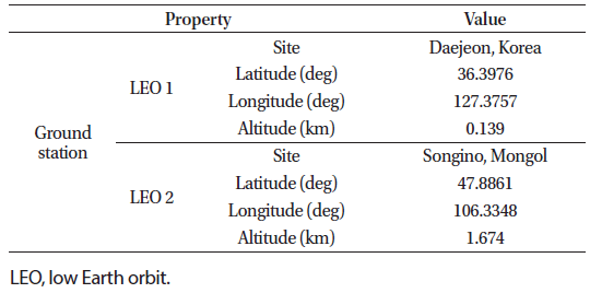
This section aims to verify which IOD method is the most appropriate, depending on the properties of observational data used. Since we need to decide which IOD method is the best for use with OWL-Net data, artificial orbits were produced that are similar to those of the Cryosat-2 and KOMPSAT-1 satellites, and artificial observation data were generated for the numerical simulations. Table 1 shows information concerning the observation ground sites, and Table 2 shows the environment simulated.
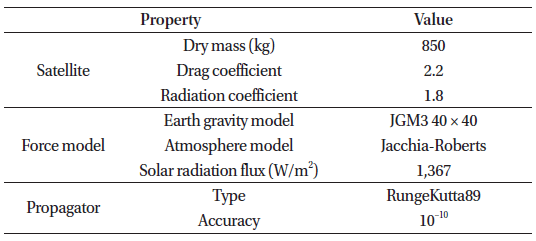
Optically observed data is in the form of topocentric RA and DEC which are derived from optical images. In this simulation, two types of artificial LEO satellite were generated to analyze the performance and property of the IOD methods. The orbital elements in the form of Two Line Elements (TLE) and observational time were set as similar to real satellites, after which the orbits were propagated for 600 sec and topocentric RA and DEC data were generated at intervals of 1 sec. The position and velocity vectors in the Earth Centered Inertial (ECI) coordinate systems were used as the true values of orbit determination. The Earth gravity model (EGM96, 40 × 40), the gravity of Sun/Moon, and the atmospheric drag model (Jacchia-Roberts) were applied for orbit propagation. The tolerance of convergence of the computed range was set to be 10–10 km. Table 3 shows the information concerning the orbital elements of the artificial satellites and the properties of the observed data used in the simulation.
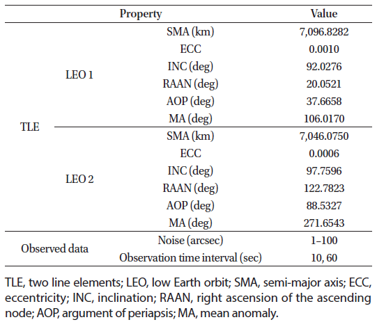
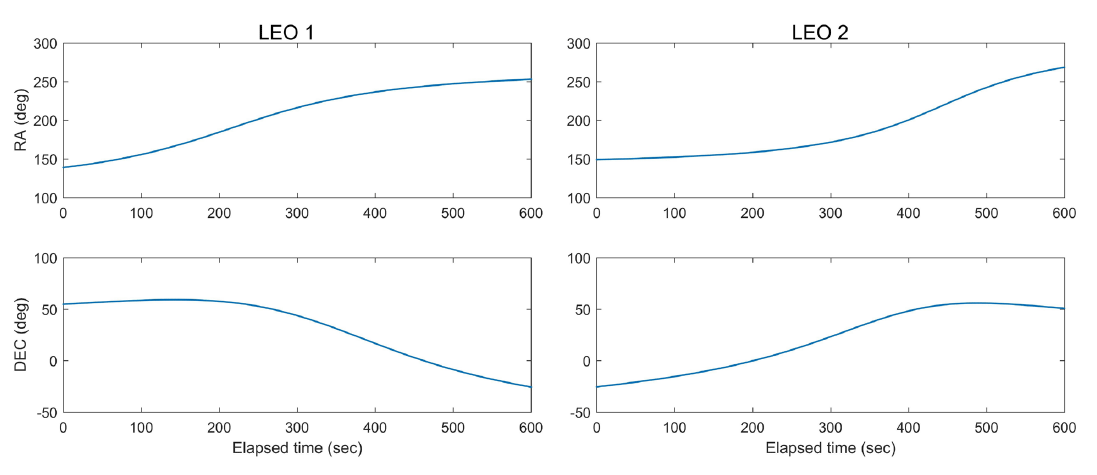
Fig. 1 shows the distribution of the RA and DEC observation data from the artificial LEO satellites over time. Three sets of RA and DEC were selected from the generated data for IOD, after which the performance of each IOD method was analyzed depending on the noise level and the observational time interval. From these simulations, the Gooding method was found to be too sensitive to the initial guess of the range, so the range value was initially guessed based on the result of the Gauss method.
Observational noise is randomly included in the observed data because of changes in the weather or system conditions. If IOD is conducted with data corrupted with noise, the accuracy of the determined orbit decreases. To assess the effects of noise on the results of IOD, we conducted a hundred Monte-Carlo simulations with artificial data that had been corrupted with Gaussian noise. The standard deviation of Gaussian distribution was set from 0 arcsec to 10 arcsec at 1 arcsec intervals, and from 20 arcsec to 100 arcsec at intervals of 10 arcsec. If noise was not included, the simulation was conducted once in order to analyze the performance of the IOD method itself. If random noise was included, simulations were conducted a hundred times to analyze the statistical performance of the IOD methods. In this case, the average of a hundred results (the position and velocity vectors at the middle observation point) was used as the result of the IOD, and the Root Mean Square (RMS) position and velocity errors were used as an indicator to demonstrate the accuracy of the IOD methods.
Fig. 2 is the result of setting the observational time interval at 60 sec and the noise level at 50 arcsec, which demonstrates the absolute error in the position and velocity vectors. While the position errors of the Gauss, double-r, and Gooding methods are less than 2 km for each axis, the result of the Laplace method is highly inappropriate for use with LEO satellites, as mentioned in section 2. The position errors produced by the Laplace method are hundreds of km on each axis. Therefore, the Laplace method is excluded in further analysis, as its accuracy is too low for any meaningful analyzation.
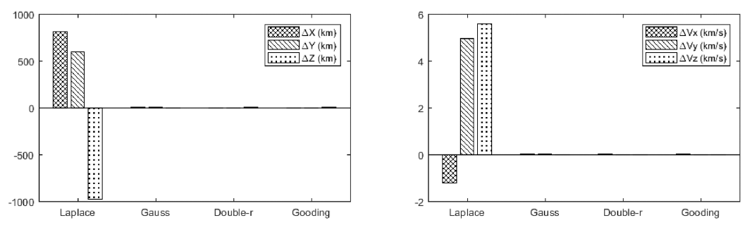
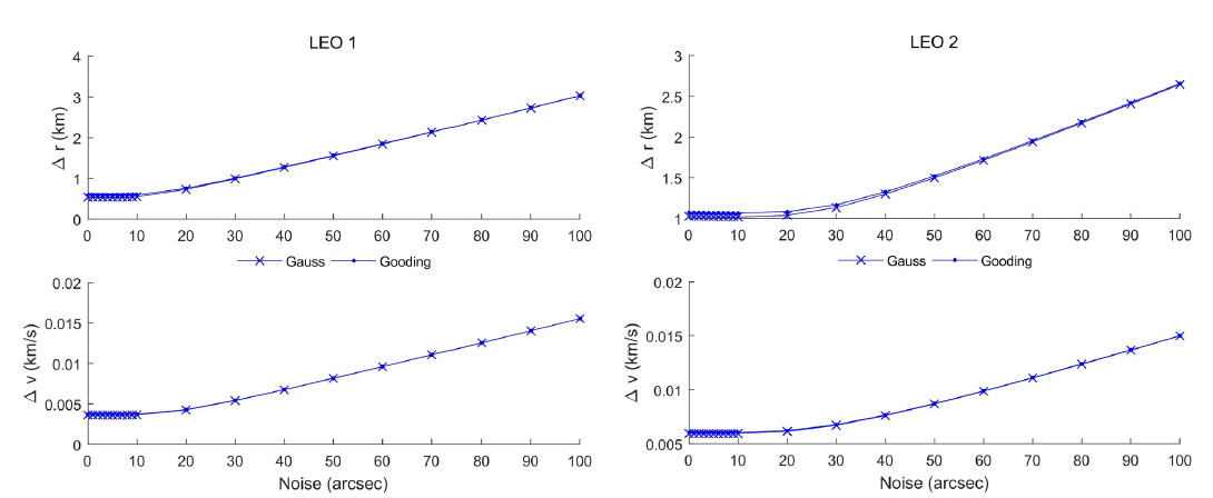
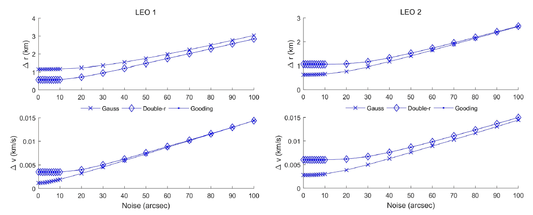
Fig. 3 shows the RMS errors in the three-dimensional position and velocity with observed data sets of 10 sec intervals, and Fig. 4 shows the errors in the observed data sets with 60 sec intervals. Fig. 3 does not include the results of the double-r method as either the position errors are hundreds of km or the method has failed to converge. Overall, the results of the Gauss, double-r, and Gooding methods show that the RMS error values for three-dimensional position and velocity tend to increase proportionally with noise level. Thus, noise level is not considered to have any effect on the differences between the IOD methods.
Three sets of RA and DEC data are required for IOD, selected from various observational time intervals. For this simulation, the observational time intervals were selected to be from 1 sec to 120 sec and the noise level was fixed at 50 arcsec. In addition to general errors such as noise and bias, the real observational data includes several errors due to the characteristics of the optical equipment or clock accuracy. The error was set at 50 arcsec to simulate the worst case where these errors are not corrected.
Fig. 5 shows the results of IOD when the observational time interval is from 1 sec to 30 sec. Under these conditions, the results of the double-r method either did not converge or produced errors of several hundred km and the results of the Gooding method also did not converge accurately, so the double-r and Gooding method are thought to be less precise than the Gauss method. This is pronounced with observational time intervals of less than 10 sec. Fig. 6 shows the results when the observational time interval is between 30 and 120 sec. From the figure, it is apparent that the errors in the three-dimensional position and velocity increase with the observational time interval when using the Gauss method. However, comparing the left part of Fig. 6 to the right, the Gauss method is most accurate when the time interval is within 40 sec for LEO 1 and within 70 sec for LEO 2. This result suggests that orbital characteristics such as altitude also affect the results of the Gauss method. However, the double-r and Gooding methods show robust results even when observational time interval increases.
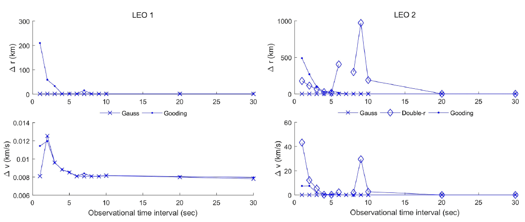
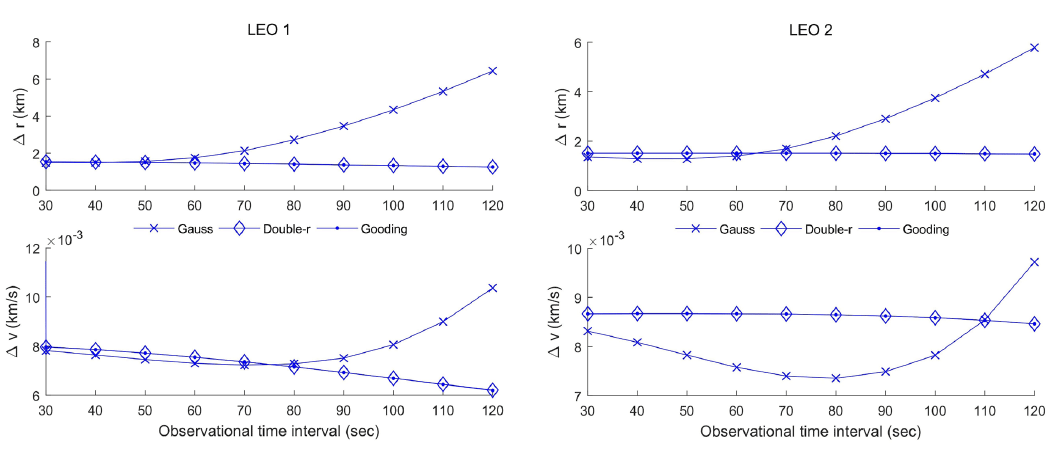
To conclude, the double-r and Gooding methods are unstable or show position errors of several hundred km in certain cases. The Gauss method is appropriate when the observational time interval is shorter than 10 sec for LEO 1, and appropriate when time interval is shorter than 60 sec for LEO 2. It is therefore suggested that the Gauss method would be the best IOD method for use with Cryosat-2 and KOMPSAT-1, as the observational data is narrowly distributed.
4. OWL-NET APPLICATION
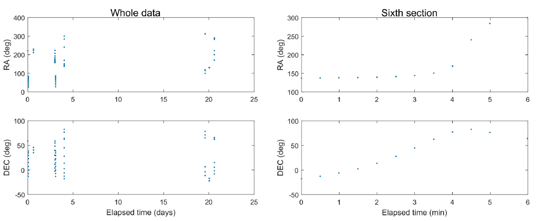
In this research, OWL-Net data for two LEO satellites, Cryosat-2 and KOMPSAT-1, were used to verify IOD methods. The file reporting OWL-Net data includes the name of the satellite and information concerning the ground site, the topocentric RA, the topocentric DEC, and the observational time. There are 75 data points in the Cryosat-2 file and 58 data points in the KOMPSAT-1 file. Each file includes the observation of multiple orbits. Only certain sections were selected for use in IOD because IOD methods only cover a single revolution. Figs. 7 and 8 show the total, and selected observational data distributions of the Cryosat-2 and KOMPSAT-1 satellites as elapsed time. One point was selected to be the middle point for IOD and IOD was conducted using a combination of all the data. After converting the position and velocity vectors of the middle point into the mean orbital elements, the average was considered to be the result of the IOD. The results were then compared with TLE from the Combined Space Operation Center (CSpOC). The Laplace method was excluded from this section because it showed highly inappropriate results with artificial LEO satellites, as mentioned in Section 2. Therefore, only the results of the Gauss, double-r, and Gooding methods were discussed.
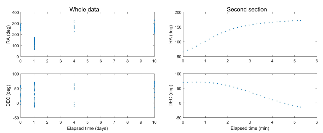
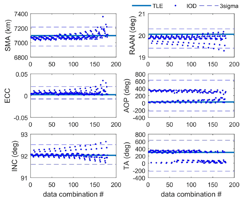
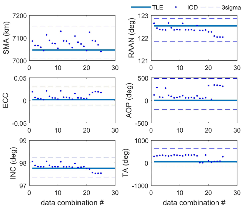
For the analysis of the results for Cryosat-2, the second dataset was selected as it contains the largest amount of data, from number 17 to number 46. The data numbered 32 was selected as the middle point to set the time intervals as evenly as possible. Specific data with errors above 3 sigma were then removed, as the properties of these data were considered to be unreliable; if these data are included, the Semi-Major Axis (SMA) of the IOD results shows a 1,000 km error compared to TLE. Table 4 and Figs. 9 and 10 show the IOD results with data combinations that exclude these unreliable data. Most of the results are distributed within 3 sigma, having similar values to the TLE data. The data numbered 45 and 46 were removed for the Gauss method, and data 44, 45, and 46 were removed for the Gooding method. Thus, the process of excluding irregular data is important, depending on the IOD method used. From Table 4, the Gauss algorithm is the most appropriate method for use with Cryosat-2 data because the errors of the determined orbital elements are the smallest relative to TLE. These results are consistent with the general characteristics of the Gauss method mentioned in Section 2.
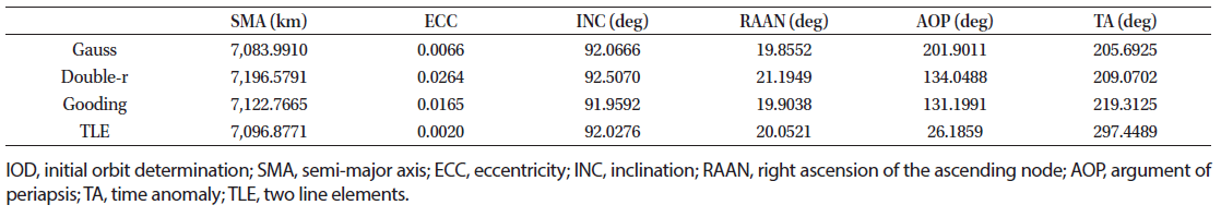
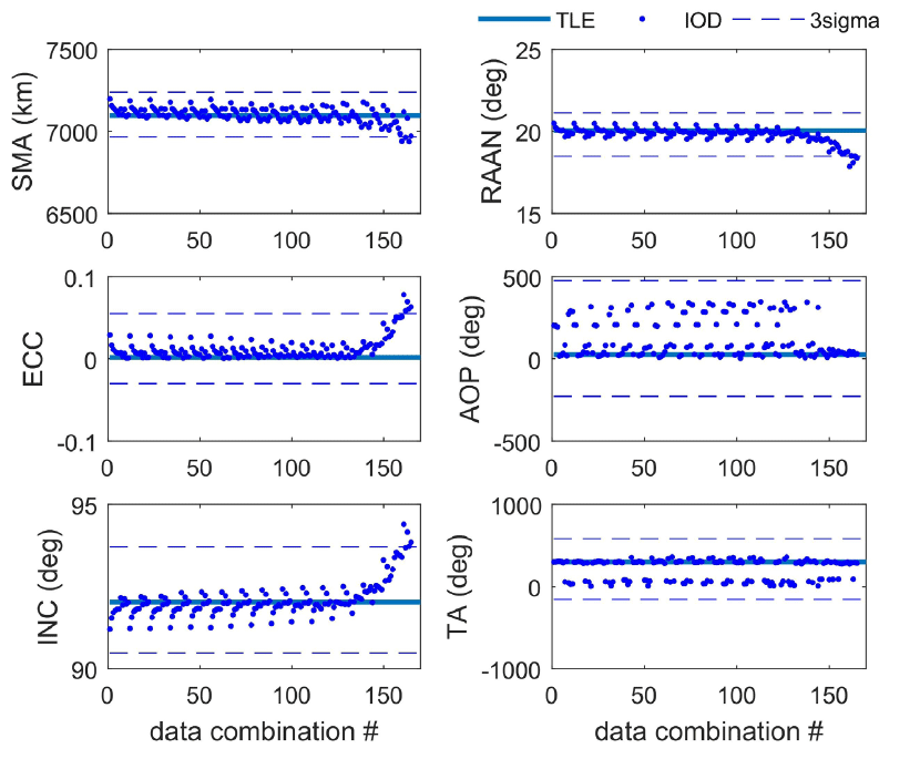
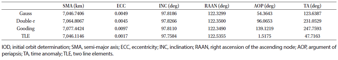
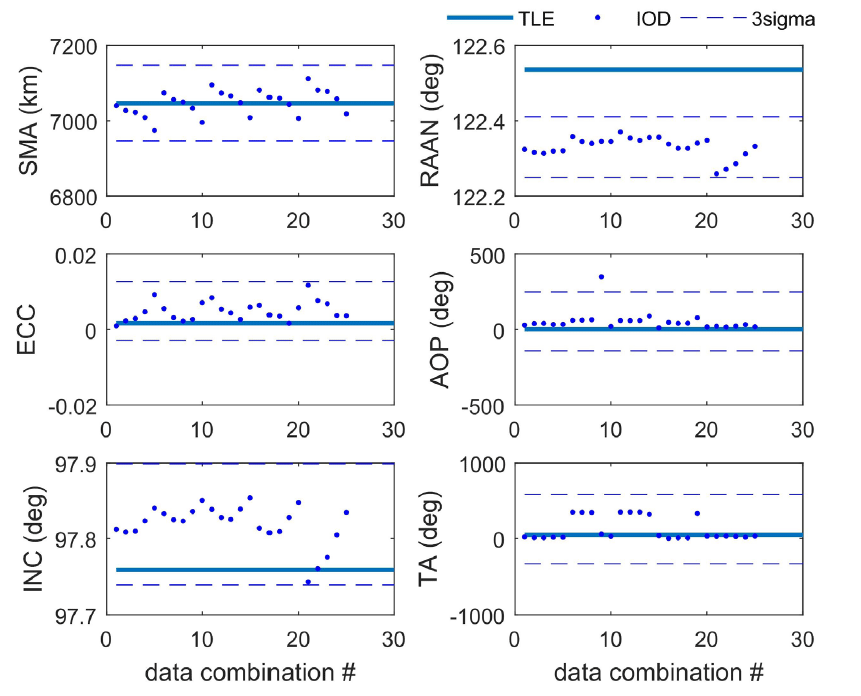
The fourth dataset was selected for analysis of KOMPSAT-1. Among the 9 data in the fourth dataset, the data numbered 18 was selected to be the middle point. Table 5 shows the results of the IOD. According to Table 5, inclination (INC) and RA of the Ascending Node (RAAN) show similar values for all methods, and the error produced by the Gauss method is the smallest in terms of SMA. The Gauss method is therefore considered the most accurate for use with KOMPSAT-1, like Cryosat-2. The reason for the large error in eccentricity (ECC), argument of periapsis (AOP), and time anomaly (TA) is that the orbit of KOMPSAT-1 is nearly circular and therefore has an ECC value close to zero, with no perigee from which to measure AOP and TA. Figs. 11 and 12 show the results of the Gauss and Gooding methods, demonstrating that most of the results are distributed within 3 sigma, which means that the results of each IOD method have a specific tendency. However, it is difficult to decide general tendencies since the number of KOMPSAT-1 data produced from a single revolution is less than that of the Cryosat-2 data.
5. SUMMARY AND CONCLUSION
In this study, observational data from artificial LEO satellites was used to analyze the characteristics of method used for IOD, and real observational data from OWL-Net was then applied to verify the analysis. The characteristics of the IOD methods were investigated using numerical simulation according to the properties of the observational data. Using the Laplace method, the position errors were found to be hundreds of km, too high for any meaningful analyzation. Using the Gauss method, the errors were lowest with observational time intervals shorter than 10 sec, and the errors were highest with time intervals longer than 60 sec, among all the IOD methods investigated. It was also apparent that the errors increase as the time interval increases. When using the double-r method it was found that the results were not likely to converge with observational time intervals shorter than 30 sec. Thus, the double-r method could only be used for time intervals longer than 30 sec, and error values were similar to the errors produced by the Gooding method. The Gooding method was found to be appropriate when the time interval is longer than 60 sec. For time intervals longer than 10 sec and shorter than 70 sec the method used needs to be decided through simulation since the IOD results depend on orbital properties. These simulation results are similar to the results of the studies that the position errors of the IOD result of LEO satellites are about several ten kilometers (Der 2012), and the probability of the double-r method failing when the observation time interval is about 10 sec or more (Schaeperkoetter 2011), and the Gauss method error is small when the observation time interval is less than about 60 sec but the error is proportional to the interval when the interval is longer than about 60 sec (Karimi & Mortari 2011).
We analyzed the properties of IOD methods by applying real observational data from two LEO satellites, Cryosat-2 and KOMPSAT-1, and then TLE data was used as a reference. The Laplace method was excluded from the analysis using real data because of the significant position errors, as mentioned in Section 3. From Tables 4 and 5, it is apparent that the SMA errors were up to several tens of km. INC and RAAN were determined with the errors of 1, 2 deg level. Significant errors were observed in AOP and TA because both satellites follow nearly circular orbits. The double-r and Gooding methods tended to fail to converge with real data corrupted with errors, as mentioned in Section 2. Overall, the Gauss method was found to be the most appropriate for finding the initial value of POD using real observational data.
For POD, an initial guess of the state vector is needed, and generally the results from IOD or verified ephemeris such as TLE and Consolidated Prediction Format are used. Accurate prediction is important because the accuracy of the POD depends on the accuracy of the initial guess. In this study, we analyzed the characteristics of the IOD methods and applied observational data with various characteristics. It is therefore possible to improve the accuracy of IOD by selecting an appropriate method according to the characteristics of observational data such as noise level and time interval.