1 INTRODUCTION
The need to develop technology for space situational awareness (SSA) initiatives is on the rise, to protect people and assets from space hazards. The main purpose of an SSA system is the surveillance and tracking of space objects that are likely to re-enter the Earth’s atmosphere, or collide with satellites and space debris. In particular, obtaining knowledge of the position and orbits of space objects is one of the most important aspects of SSA (Donath et al. 2010; Kalden & Bodemann 2011; Kennewell & Vo 2013). In recent years, surveillance systems based on radar have provided more comprehensive information regarding space objects under observation, compared to that obtained by optical systems. Radar systems have high detection probabilities for objects in low earth orbit (LEO) by two way distance due to the active illumination they perform using electromagnetic radio waves. In addition, radar systems are advantageous as they can be operated independent of meteorological and daytime conditions. Hence, radar systems configured for SSA are required for the assessment of the general condition of space objects, and to perform risk assessments for reentering space objects.
According to the box scores of a satellite situation report issued on October 18 2017, the United States space surveillance network (SSN) tracks 18,780 orbital space objects above 10 cm in size. Of these, only 1,892 are active satellites (Space- Track 2017). The SSN consists of a worldwide network of space surveillance sensors—radars and optical systems (Ender et al. 2011). Radar instruments, such as the Eglin AN/FPS85 phased-array radar, the PAVE PAWS phased-array warning system, the L-band Cobra Dane system, and the two radars at Massachusetts Institute of Technology (MIT)’s Millstone hill and Haystack observatory complex, are included in this network (Halte 2012). An upgraded Space Fence system is also being developed by the US Air Force (Haines & Phu 2011; Haimerl & Fonder 2015). The improved Space Fence system, with extremely powerful S-band radar, is expected to be able to detect the returns of smaller objects, and to increase the number of observations, enabling the compilation of a more accurate and complete catalog of these events. The European Space Agency (ESA) initiated an SSA program in 2009, which includes the use of existing European and ESA assets, and development of future radar systems, for detecting and surveying all objects on the order of one decimeter in LEO (Ender et al. 2011). Existing radar sensors in Europe include the Fylingdales station in the UK, the Norwegian Globus II radar, the French GRAVES system, and the German FGAN radar (Klinkrad et al. 2008). The Fraunhofer Institute for High Frequency Physics and Radar Techniques (FHR) has been commissioned by the German Space Administration (DLR), on behalf of the German Federal Government, to develop a phased-array radar system, to monitor space objects in LEO. This project, called the german experimental surveillance and tracking radar (GESTRA), will support the German Space Situational Awareness Center in generating a catalogue of orbital data for objects at altitudes of less than 3,000 km (Wilden et al. 2016; Wilden et al. 2017).
In Korea, the development of SSA systems has been considered, according to the preparedness plan for space hazards (Choi et al. 2014; Choi et al. 2015a, 2015b). At present, the optical wide-field patrol network (OWL-Net), with five optical telescopes in different locations around the world, is the only infrastructure for Korean SSA programs (Park et al. 2015; Lee et al. 2017). However, due to the dependence of this network on weather conditions and observation time, it is not reasonable to use optical systems alone for SSA activities, as they have limited operational availability (Bae et al. 2016). The development of radar systems should thus be considered, to create an efficient SSA system with currently-available technology. Accordingly, the National Space Situational Awareness Organization (NSSAO) initiated a conceptual study of the operation of a space objects observation system using the existing optical system, and the radar system necessary for efficient operation. A preliminary study considering the development of efficient SSA radar systems is being conducted by the NSSAO. The work summarized in this paper was conducted as part of this study, to analyze the performance of radar systems in detecting and tracking space objects in LEO. This paper presents a comparative study of several reference radar parameters for various frequencies, as well as design of the power budget, by means of simulation. These results provide the basis for development of future SSA radar systems.
2 SPACE SITUATIONAL AWARERNESS SYSTEM
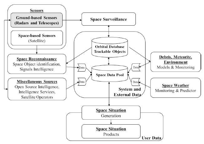
The purpose of an SSA system is to observe, analyze, and predict the location of natural and man-made objects in orbit around the Earth. Fig. 1 illustrates a schematic block diagram of the typical architecture of an SSA system (Bobrinsky & Del Monte 2010; Kalden & Bodemann 2011). The overall SSA system comprises sensors, database, and user interface. The core of this system is the database of trackable space objects, which must be updated continuously. The data is based on observations from ground-based and space-based sensors, and information from external sources from international cooperation networks. Table 1 provides a summary of representative sensors, available currently, which are capable of performing SSA tasks.
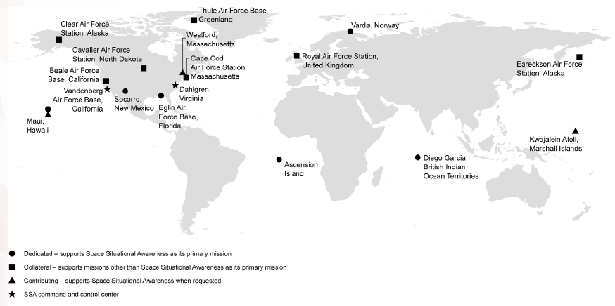
At present, the only nation with an operational space surveillance capability, and with a routinely updated space object catalog, is the USA. The SSN, which is conducted by the Joint Space Operations Center (JSpOC), is currently the single best source of SSA information in the world. Fig. 2 shows the global network of 30 space surveillance sensors, including ground-based radars, ground-based optical telescopes, and space optical sensors, used to observe objects (Weeden et al. 2010; Baird 2013; Kennewell & Vo 2013). Ground-based radars such as Globus II, the AN/FPS-85 space track radar, and the Haystack ultra-wideband satellite imaging radar (HUSIR), also contribute sensors to the SSN (Walsh 2013). Radar systems have high detection probabilities at large and very large ranges, with the ability to penetrate cloud cover. These characteristics are required for the assessment of the space situation, and physical characterization of space objects, as well as for risk assessment of re-entering space objects. When phased-array radars are used as sensors, they can track multiple satellites simultaneously, and scan large areas of space in a fraction of a second. Conventional radars with mechanically steered reflector antennas can only track one or a few objects with high precision (Chatters IV et al. 2009; Weeden et al. 2010; Ender 2011; STRATCOM 2017). Space Fence, the new S-band ground-based radar system on Kwajalein Atoll in the Marshall Islands, is expected to provide unprecedented detection sensitivity, coverage, and tracking accuracy. To accommodate Space Fence, JSpOC has initiated the process of upgrading major hardware and software systems. The completed system will be expected to detect and track as many as 150,000 additional man-made objects as small as the size of a golf ball (Haines & Phu 2011; Haimerl & Fonder 2015; Loomis 2015).
In addition to ground-based radars, optical systems are essential contributors to the SSA mission. The ground-based electro-optical deep space surveillance (GEODSS) system plays a vital role in tracking space objects, particularly those in deep space. The Air Force Maui Optical Station (AMOS) is a state-of-the-art electro-optical facility for detecting and tracking orbital debris. AMOS includes a 1.6-meter telescope, and a 3.67-meter advanced electro-optical system (AEOS) telescope with an adaptive optics (AO) system. This system can perform surface characterization and identification of space objects (Africano et al. 2004).
In Europe, SSA program was approved in November 2008, during the ministerial level ESA council (Bobrinsky & Del Monte 2010; Tsujino 2012). Following a feasibility analysis of possible European SSA systems, conducted as the initial preparatory phase of the program, activities in the space surveillance and tracking (SST) segment, in the second phase of the program, are currently in progress (Donath et al. 2010; Fletcher 2010). Tasks performed by the European space surveillance system (ESSS) comprise the following elements: full coverage of objects in LEO and geostationary earth orbit (GEO), autonomous build up and maintenance of a catalog of all observable space objects, estimation of orbit maneuvers, and detection of on-orbit break-up events (Klinkrad et al. 2007; Donath et al. 2010). Although Europe does not currently have a network of dedicated SSA sensors, it has access to several radar and optical facilities. The French GRAVES system determines orbital element sets using measurements of direction angles, Doppler and Doppler rates, from a large number of targets, performed simultaneously using four planar phased-array antennas, with dimensions of 15 m × 6 m each (Michal et al. 2005; Klinkrad et al. 2008). The German TIRA system, which has a parabolic dish antenna with a 34-m diameter, uses the L-band for tracking at 1.333 GHz, and the Ku-band for inverted synthetic aperture radar (ISAR) imaging at 16.7 GHz (Klinkrad et al. 2008). The Ku-band system generates high resolution radar images of space objects at a distance of up to 20,000 km, which enables identification and technical analysis. The optical sensors operated by Europe are primarily used to observe objects beyond LEO altitudes. However, the Space Debris Telescope on Tenerife, which has a 1-m aperture and a 0.7° field of view (FoV), and the Zimmerwald laser and astrometry telescope (ZIMLAT), with a 1-m aperture and a 0.5° FoV, cover only 120° and 100° sectors of the GEO ring, respectively (Klinkrad et al. 2008).
Space-based optical telescopes provide a number of advantages over ground-based systems, primarily, the absence of interference from weather and atmosphere, and the mitigation of limitations relating to the time of day, and are increasingly being considered as an important component of SSA systems. The space-based surveillance system (SBSS) program is a planned constellation of satellites for tracking space objects in orbit, and accomplishing space situational awareness for future space control operations. This satellite system, with space-based visible (SBV) sensors, will operate constantly (24 hours a day, 7 days a week).
3 RADAR PERFOMANCE ANALYSIS
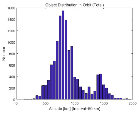
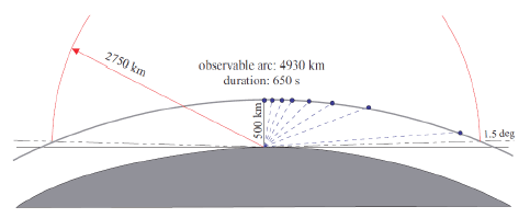
Radar systems for use in SSA initiatives are required to be able to detect space objects up to a height of 2,000 km, because, as shown in Fig. 3, approximately 78 % of trackable space objects are distributed in this region. The maximum range required to observe objects at this height is a function of the maximum elevation of the system (Ender et al. 2011; Liebschwager et al. 2013; Eilers et al. 2016). Fig. 4 illustrates how the maximum range of the radar affects the observable altitude. The requisite operational range of the radar system is determined from the desired range of elevation angles, and the maximum orbit altitude.
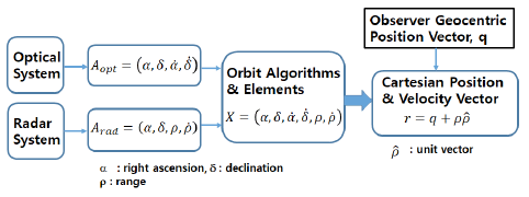
In general, the position of an orbiting object can be represented using a topocentric coordinate system, with the angles defined as right ascension (α) and declination (δ). With optical systems, the vector representing the observed data is given, without range, ρ, and range rate, , as , where the ̇ operator indicates a rate of change. In contrast, with radar systems, the vector representing the observed data is given as . To determine orbital parameters, the observed data must be represented as . At observer position vector q, the Cartesian position vector of an orbital object is , where is a unit vector. Therefore, orbital elements can be calculated from the Cartesian state vectors, using the orbit algorithms shown in Fig. 5.
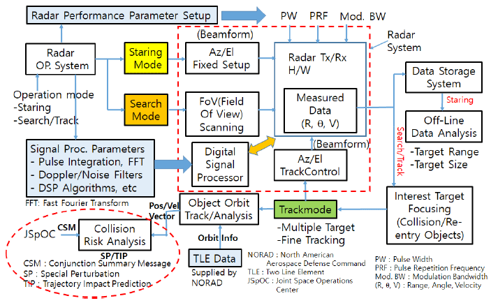
Three different utilization modes can be defined for SSA radar, depending on the operation scenario. In ‘Staring mode’ all objects passing through the antenna beam width, with the antenna position fixed to a certain azimuth and elevation angle, are detected. In ‘Search mode’, all space objects passing through the sensor’s FoV during scanning can be detected. If some objects of interest are identified during search mode, ‘Track mode’ is activated, where the radar beam focuses on designated objects by continuously controlling the antenna direction. More accurate position and angle data can be obtained for tracked objects using this mode. Fig. 6 depicts a flow diagram illustrating control and selection of the radar operation scenario. We define parameters controlling the observability of space objects, including pulse width (PW), pulse repetition frequency (PRF), and modulation bandwidth (Mod. BW) as well as parameters for signal processing. This conceptual scenario can lead to efficient operation of SSA radar systems.
In general, there are two types of radar configuration: monostatic and bistatic configurations. In the monostatic configuration the transmitter and receiver are situated in the same location, whereas in the bistatic configuration, they are situated in different locations, separated by a considerable distance. To estimate radar performance in terms of the maximum range, we consider the detection probability and beam extension in different frequency bands, for a given target position. As we used the radar range equation to estimate the maximum theoretical detection range for a particular target, it is fundamental to determining radar performance (Patyuchenko et al. 2011).
The performance of a radar system can be estimated using the simplified radar range equation for a monostatic pulsed radar (Skolnik 1980). For such configurations, the received power, Pr, is expressed as,(1)
where Pt is the peak power of the transmitter, Gt is the gain of the transmitting antenna, Gr is the gain of the receiving antenna, λ is the wavelength of the radio wave, σ is the radar cross section (RCS), Ls is the loss factor of the total system, and Lp is the propagation loss due to the absorption of the electromagnetic wave by O2 and H2O molecules in the atmosphere, which is dependent on the radar frequency. |F|4 is the propagation factor, where , which is the ratio of the actual magnitude of the electric field to the magnitude of the electric field in free space, R is the radar range to the target, and Gp is the gain from signal processing, which is usually implemented in the form of a pulse integration technique.
The noise power, Pn, is expressed as,(2)
where k is Boltzmann’s constant (1.38 × 10⁻²³ J/K), Ts is the noise temperature of the system, which is usually defined as Ts = T0F, where T0 is 290 K and F is the noise factor of the receiver, and Bn is the receiver’s noise bandwidth. The noise figure of the receiver, NF, is expressed in dB unit as NF = 10 log10(F). It should be noted that the noise factor, F, is different from the propagation factor, |F|.
The signal-to-noise ratio is defined as,(3)
The radar constant, K, can be determined by the parameters of the hardware subsystem of the radar system as follows:(4)
From the radar range equation, the SNR can be expressed in terms of K as follows:(5)
Alternatively, the maximum radar range, Rmax, can be expressed as,(6)
where SNRmin is the minimum SNR.
The maximum detection range can thus be computed as a function of RCS. RCS is dependent on the radar frequency and the size of the target, which is usually modeled as a conductive sphere with radius, r. For space surveillance and tracking radar systems, the NASA size estimation model (SEM), which is based on the results of measurements performed in the 2.4 GHz–18 GHz frequency range (encompassing the S, C, X, and Ku bands), is typically used for calculation of the RCS. The RCS of a sphere is calculated differently in three scattering regions: Rayleigh, Mie, and optical. NASA SEM curves are calculated as follows (Stokely et al. 2006):(7a)(7b)(7c)
where x = d/λ, d is the diameter of the object, and z = σ/λ2. In the Mie resonance region, the smooth function, g(z), can be expressed using curve fitting.
In this paper, to analyze the performance of the radar system, we defined detection of a target with a diameter of 1 m at a distance of 2,000 km, as the benchmark sensitivity. Key radar reference parameters for all frequency bands considered are shown in Table 2. Atmospheric attenuation was assumed to be constant above the troposphere. The values of atmospheric attenuation are 1.2 dB, 1.5 dB, 1.7 dB, 2.4 dB, and 5.5 dB at 1.3 GHz, 3.0 GHz, 5.5 GHz, 10 GHz, and 16.7 GHz, respectively (Mahafza & Elsherbeni 2003). We defined the signal to noise ratio of a single pulse, SNR1, using a 1-m2 RCS at a range of 1,000 km.
For phased-array antennas with an element spacing of λ/2, the antenna gain and 3-dB beamwidth can be estimated using the following formulas (Skolnik 1980):(8)(9)
where the units of θ3dB are in degrees, N is the number of elements, and η is antenna efficiency.
When η = 0.65 and N = 5,000, the antenna gain is 40 dBi, with a beamwidth of 1.4°. A peak transmit power of 100 kW can be obtained with a single element power, P0, of 20 W, since Pt = N × P0.
The probability of detection, Pd, can be calculated in terms of SNR1 and the probability of false alarm, Pfa. The approximate relation between these parameters is (Mahafza & Elsherbeni 2003):(10)
The requisite SNR for Pd = 80 % when Pfa = 10−6, is 12.6 dB.
Fig. 7shows the results of simulations using the reference radar parameters. From this figure, we can observe the frequency dependence of detection ability for the same set of parameters. Although the detection range decreases with frequency, radar systems operating at higher frequencies have some advantages, such as the reduced dimensions of the hardware, and detection of smaller target sizes in some applications, due to the shorter wavelength.
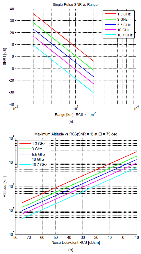
Table 3 summarizes the reference radar performance at different frequencies. A higher transmit power and antenna gain is necessary when increasing the frequency. However, as increases in power and antenna gain are challenging problems in the relevant frequency bands, some technical compromises must be made.
The power budget was designed based on the reference performance analysis, by taking into account practical radar components. Although we considered the L-band frequency in this paper, the same method can be applied for radar systems operating at other frequencies. We assume a phasedarray radar system, which has many advantages compared to conventional radars with large parabolic antennas. These systems allow the surveillance of large angular sectors in a short amount of time, and can detect and track numerous targets simultaneously, offering multi-functional operation. It has been suggested that continuous surveillance of LEO can only be guaranteed using high performance groundbased phased-array systems (Ender et al. 2011).
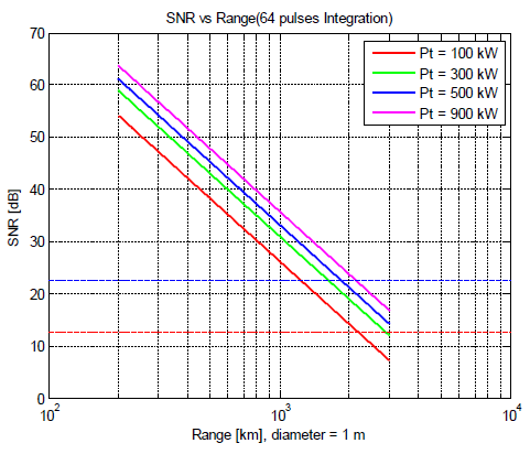
An example of a power budget design is summarized in Table 4. While Gt was fixed to 40 dB, P0 was increased from 20 W to 100 W, delivering a total peak power of 500 kW. The receive antenna, with the increased gain, is usually separated from the transmit antenna, for bistatic or pseudo-monostatic operation. The signal processing techniques used in radar systems are also very important. The most commonly used method is pulse integration, which can be coherent or noncoherent. In space surveillance radars, 16 or 64 pulses are typically used for non-coherent integration, which gives processing gains of 9.5 dB and 13.3 dB, respectively (Mahafza & Elsherbeni 2003). The average transmit power, Pav, is calculated as Pav = Pt × τ × PRF, where PRF is the pulse repletion frequency and τ is the pulse width. Hence, a longer pulse width yields a higher average power. We included an additional SNR margin of 10 dB, to account for unmodeled losses. As incrementing individual parameters may be accompanied by high costs, a tradeoff analysis of cost and performance is needed.
The results of simulations are shown in Fig. 8. As can be seen in this figure, the maximum range of 2,000 km can be achieved for a target size of 1 m2 with a transmit power of 900 kW. The detection capabilities of the radar system, in terms of range and target diameter, can be estimated easily, using Table 5. For example, for a range of 1,000 km and a target diameter of 50 cm, the SNR is 27.3 dB when Pt = 500 kW. As the SNR is greater than the detection threshold of 22.6 dB (blue dotted line in Fig. 8), the target size can be detected at 1,000 km for the given radar parameters. Doubling the detection range reduces the SNR by 12 dB, since SNR is inversely proportional to the fourth power of the range.
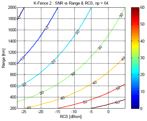
An SNR contour map with respect to range and RCS is shown in Fig. 9. The range extends from 200 km to 2,000 km, with 5 km intervals, and RCS is plotted from −27.07 dBsm to 4.97 dBsm, corresponding to object diameters of 5 cm to 2 m, which are separated by 5 cm intervals. The radar parameters are, Pt = 900 kW, Gt = 40 dBi, Gr = 43 dBi, and pw = 2 ms, at a frequency of 1.3 GHz. The processing gain, Gp, was set to 13.3 dB. Since the detection threshold, including the 10 dB margin, was calculated to be 22. 6 dB, the detection region is to the right of the 20-dB SNR contour line. This map can thus easily illustrate radar performance in terms of range and the size of the space object or RCS.
4 CONCLUSION
The behavior of a radar system for detecting and tracking space objects was simulated, to analyze its detection capability in terms of frequency, transmit power, and target size (measured in diameter). Two principal types of system are available with current radar technology: systems with mechanically steered reflector antennas, and phased-array antennas. Continuous space situational awareness can be guaranteed using a high-performance ground-based phased-array radar system with electronic beam-steering, enabling tracking of multiple space objects simultaneously. In general, a higher transmitted power and antenna gain results in the detection of smaller space objects, and a longer detection range. This demonstrates that the detection performance of a radar system is heavily dependent on hardware. Therefore, for an efficient SSA system using current technology, a relevant strategy that takes cost and performance into consideration is needed.
We applied non-coherent pulse integration as a simple radar signal processing technique, during simulation. The results of power budget analysis showed that the maximum detection range of 2,000 km could be achieved with a transmit power of 900 kW, transmit and receive antenna gains of 40 dB and 43 dB, respectively, a 2-millisecond pulse width, and a signal processing gain of 13.3 dB, at a frequency of 1.3 GHz. The SNR required for an 80 % probability of detection with a false alarm rate 10−6, was assumed to be 12.6 dB. An additional SNR margin of 10 dB was included, to account for unmodeled losses. In order to further improve the SNR, coherent signal processing techniques, such as pulse compression, constant false alarm rate (CFAR) detectors, and other advanced algorithms, will be necessary in the base band, which usually require complex systems, and incur higher costs. The key parameters of the radar system were designed through a performance analysis and tradeoff study. We also showed that phased-array radar systems are the most suitable technology for detecting and tracking space objects in combination with OWL-Net. These results will be expected to be used for the conceptual design of SSA radar system. In particular, the analysis of the detection capabilities of the radar can provide guidelines for the development of radar systems for SSA programs.