1. INTRODUCTION
The mesosphere and lower thermosphere (MLT, 85-100 km) region is modulated on a decadal time scale by factors originating from both the upper and lower atmosphere. For instance, MLT temperature is thought to be positively correlated with solar activity. Long-term variations of gravity waves also affect MLT temperature (Hoffmann et al. 2011;Jacobi 2014). Notably, cooling in the MLT region induced by increased carbon dioxide has been predicted by previous studies (Berger & Dameris 1993;Portmann et al. 1995;Akmaev & Fomichev 1998, 2000;Akmaev et al. 2006).
Studies using ground-based observations in mid-latitude regions have reported systematic long-term variations of MLT temperatures. She et al. (2009) estimated a solar response of 4 K/100 solar flux units (SFU) and a cooling trend of -6.8 K/ decade at the 91 km level obtained from Na lidar observations over Fort Collins (41°N, 105°W) during 1990-2007. However, Mt. Pinatubo injected a considerable amount of volcanic ash into the atmosphere, up to the stratosphere, and induced a substantial increase in MLT temperature which lasted for several years after the eruption in 1991 (She et al. 1998). After subtracting the volcanic effect, She et al. (2009) suggested that the solar response and long-term trend may be corrected to 6 K/100 SFU and -0.28 K/decade, respectively. Later, She et al. (2015) reported a slightly greater cooling trend (-1.0 K/ decade) excluding the volcanic effect for a longer period of 1990-2014.
Offermann et al. (2010) reported a significant cooling trend of -2.3 K/decade from OH rotational temperatures over Wuppertal (51°N, 7°E) f2008. However, they noted a break in the trend in the mid-1990s and subsequently estimated trends of -0.8 K/decade and -3.4 K/decade for the periods 1988-2000 and 1996-2008, respectively.
Bittner et al. (2002) and Lowe (2004) found weak or insig-nificant cooling trends from OH rotational temperatures in the 1980s-2000s, compared to the more significant cooling (-2.2 K/decade) over Zvenigorod (56°N, 37°E) reported by Perminov et al. (2014) for the period 2000-2012. Other studies on the long-term trends of MLT temperature are summarized in Beig (2011).
In this study, we derived the OH rotational temperatures over the Apache Point observatory (APO, 32°N, 105°W) using spectra of the Sloan digital sky survey (SDSS) for the period 2000-2014, and analyzed the solar response and long-term trend of OH temperatures.
2. DATA AND METHODS
In the OH airglow layer centered at 87 km, vibrationally excited OH radicals are produced by the reaction of H with O3:
where ν′ represents vibrational energy levels. The vibrationally excited OH radicals, before emitting OH airglow, collide with ambient atmospheric molecules in the 87 km altitude region so frequently that a Boltzmann distribution can be assumed for the population among the rotational energy levels. Thus, the OH rotational temperature can represent the atmospheric temperature at the OH airglow layer (Sivjee & Hamway 1987).
The OH rotational temperature can be derived from the ratio between the intensities of two rotational emission lines with different upper rotational states. We calculated the OH rotational temperature using the following equation (Phillips et al. 2004):
where h is Plank’s constant; c is the speed of light; k is Boltzmann’s constant; Fa and Fb are rotational energy term values, Ia and Ib are rotational line intensities, and Aa and Ab are Einstein coefficients of the upper rotational states. In this study, we utilized a dataset of OH airglow line intensities to determine OH rotational temperatures, derived from an astronomical spectrograph used in the SDSS project. The SDSS is an astronomical survey designed to produce a three-dimensional map of the universe. SDSS observations have been carried out at the APO since April 2000. During the first survey period, 2000-2008, the SDSS utilized SDSS-I/II spectrographs, which were connected by 640 light fibers, each 3’’ diameter, from two plates on the focal plane of a large telescope. A single observation generated 640 spectra with a spectral range of 3,800 -9,200 . At least 32 atmospheric spectra were included in those 640 spectra, to subtract atmospheric effects from the measurements of stellar intensities. More detailed information on the SDSS-I/II spectrograph is included in Stoughton et al. (2002). Since September 2009, a new spectrograph, the baryon oscillation spectroscopic survey (BOSS), has been operating with new grating, charge-coupled device (CCD), and 2’’ diameter light fibers. The number of maximum spectra increased to 1,000 and more than 70 atmospheric spectra were ÅincludedÅ. The spectral wavelength range also expanded to 3,600 -10,400 (see Aihara et al. (2011) for more details of the BOSS spectrograph).
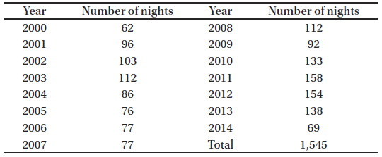
In this study, we used SDSS atmospheric spectra for a 15-year period since 2000. The observation period excluded the July to August maintenance period (DOY 190-230, roughly). The nights available for OH temperature determination are listed in Table 1.
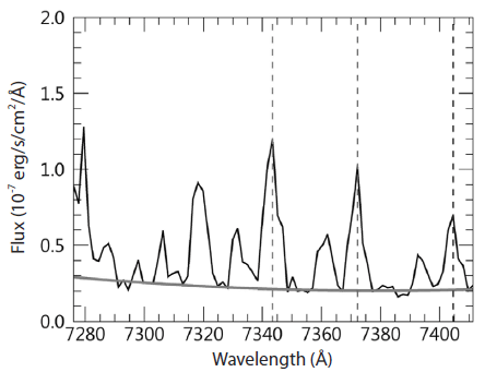
We selected OH(8-3) P-branch emission lines from the SDSS sky spectra to retrieve OH rotational temperatures. The spectroscopic parameters of OH(8-3) P1 (3), P1 (4) and P1 (5) emission lines are presented in Table 2. To avoid accidental contamination from nearby stars, we excluded the fibers whose fluxes exceeded four times the average flux at the central wavelengths of the three lines. Spectra of all sky fibers except these (usually one or two out of thirty-two sky fibers) were combined for each wavelength and divided by the number of added fibers. Fig. 1 shows a combined sky spectrum in the 7,275Å-7,410Å range of the OH(8-3) P-branch. The baseline of the combined spectrum is removed by the standard second polynomial fitting method. The line intensities were computed by adding the Gaussian function within ±1.5Å of the central wavelength, after Gaussian fitting the emission feature within ±3Å of the central wavelengths.
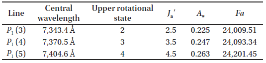
By applying the measured line intensities to Eq. (2), we determined OH rotational temperatures. The term values and Einstein coefficients of the P1 (3), P1 (4), and P1 (5) lines were adopted from Coxon & Foster (1982) and Langhoff et al. (1986), respectively, and are listed in Table 2.
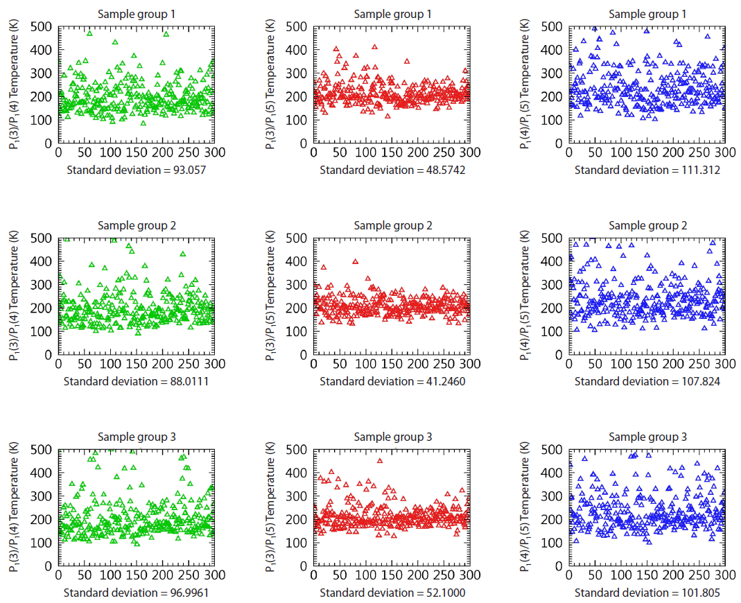
Temperature determination was carried out using three pairs from the P1 (3), P1 (4), and P1 (5) emission lines in three sample groups, resulting in nine temperature sample groups. Each sample group was composed of 300 randomly selected spectra. The sample temperatures are presented in Fig. 2. The P1 (3)/P1 (5) temperature samples have the smallest standard deviations among all the sample groups. Accordingly, we adopted the P1 (3) and P1 (5) pair for further analysis.
A microwave limb sounder (MLS) is onboard the Aura satellite that was launched by NASA in July 2004. It has sun-synchronous polar orbit with an inclination of 98° and a height of 705 km. The MLS observes the profiles of various atmospheric parameters, including the temperature from the limb thermal radiation (Schwartz et al., 2008).
For comparison with the SDSS temperatures, we utilized the nighttime mean of the MLS temperatures measured during 00-06LT over 32°N±5°, 104°W±5° at 0.00464 hPa level (approximately 88.5 km), which is near the OH airglow layer for the period 2004-2014.
3. RESULTS AND DISCUSSION
Fig. 3 shows the nightly mean SDSS and MLS temperatures and their 27-day running averages. Although the SDSS temperatures show significant scatter and gaps due to the summer maintenance period, they exhibit somewhat lower temperatures in summer than in winter. Conversely, MLS temperatures clearly show the summer minimum thanks to the continuous data stream. We also note that the average ratios of SDSS to MLS temperatures increased rather abruptly by ~1.4 % (approximately 2.75 K) after 2009. Instrument replacement in the summer of 2009 may have caused the systematic differences in temperature before and after 2009. We corrected the systematic change in SDSS temperatures after 2009 by multiplying by a scaling factor of 0.98. The scaling factor was computed as the ratio between the yearly average ratios of SDSS to MLS temperatures one year before and after the instrument replacement, based on the assumption that the ratio of SDSS to MLS temperatures would not change in the case of no instrument replacement. The scaled temperatures are shown, for the years after 2009, in Fig. 3. The difference between the SDSS and MLS temperatures is larger during summer than during winter, while the scatter of SDSS temperatures is almost the same for both seasons, as shown in Fig. 2. This implies that the difference between SDSS and MLS temperatures is not simply due to the observational or instrumental limitations of SDSS, and thus will be treated as such in our analysis. We overlapped all SDSS and MLS temperatures as a one-year time series and regarded their 27-day running averages as the seasonal variation in mesospheric temperatures over the APO.
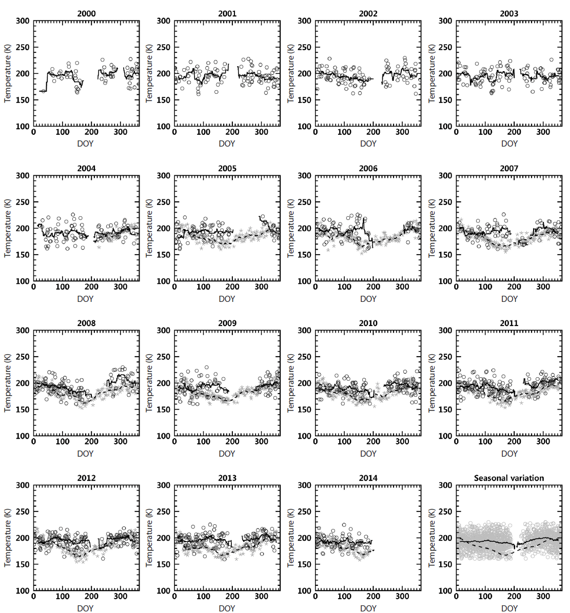
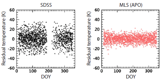
Fig. 4 shows the residual temperatures after subtracting the seasonal variations. The larger residual for SDSS than for MLS may be partly due to the small field of view of the SDSS telescope observation, which samples a smaller portion of the atmosphere than the MLS. Thus, the larger residuals do not necessarily indicate a lower quality of the SDSS temperatures, but uncertainties in the representation of average atmospheric temperature may be larger. Although the larger dispersion of SDSS residuals weakens the value of the SDSS dataset, the long range and large number of data points ensure its validity for the analysis of solar responses and long-term trends.
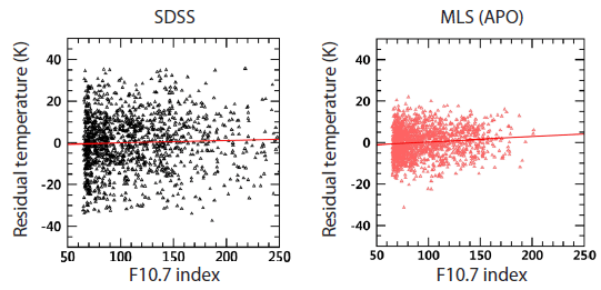
Residual temperatures over the APO, located at mid-latitudes, still show positive correlations with F10.7. The fitted slopes of SDSS and MLS residuals, as shown in Fig. 5, are 1.2 K ±0.8 K/100 SFU and 2.7 K ±0.6 K/100 SFU, respect-ively. The errors in the slope represent one standard deviation from the slope fitting. The standard deviations from the fitted line are 13.5 K and 7.0 K for the SDSS and MLS temperatures at the APO, respectively. If the correction factor of 0.98 is not applied to the SDSS temperatures after 2009, the solar response decreases to 0.8 ±0.8 K/100 SFU. This is because the enhanced temperatures measured after instrument replacement in 2009 contributed predominantly to the slope during the solar minimum. Other studies in northern mid-latitude regions report a solar response of 3 K ~ 5 K/100 SFU (She et al. 2009;Offermann et al. 2010;Perminov et al. 2014). Note that the latitudinal coverage of these studies is 40°-60°N, at least approximately 10° higher than the APO. The solar response over the APO derived in this study is in line with those of other studies at mid-latitudes. We subtracted the solar response from residual temperatures for the analysis of long-term trends.
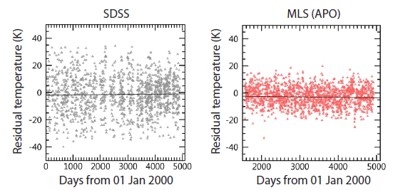
The long-term trends of mesospheric temperatures were examined by linear regression fitting between the time and the solar response removed residual temperatures. Fig. 6 shows linear regression fitting of SDSS and MLS residual temperatures with trends of 0.7 ±0.9 K/decade and -1.4 ±0.7 K/decade, respectively. Again, the errors are one standard deviation from the slope fitting. Both fitted slopes have uncertainties that are too large to interpret as a cooling trend at this site.
4. SUMMARY AND CONCLUSION
The seasonal variation, solar response, and long-term trend of mesospheric temperatures were derived by analyzing the atmospheric OH spectra observed by the SDSS during 2000-2014 at the APO (32°N, 105°W). The same analysis was performed for mesospheric temperatures at ~88 km over the APO measured by MLS/AURA for 2004-2014. Seasonal variations were determined from the 27-day running averages of the temperatures of the same days in a year. The SDSS and MLS temperatures followed the typical annual variation of mesospheric temperatures. Solar responses of 1.2 K ± 0.8 K/100 SFU and 2.7 ±0.6 K/100 SFU were found in the SDSS and MLS residual temperatures after the seasonal variations were subtracted. The estimated solar responses are consistent with other studies.
After removal of the solar responses, the trend analysis of the SDSS and MLS residual temperatures resulted in 0.7 K ± 0.9 K/decade and -1.4 K ± 0.7 K/decade, respectively; their large errors may disregard them from being significant cooling trends. The finding of an insignificant cooling trend over the APO in this study should be regarded as an independent check for climate change research since the SDSS project provides a long-term database of OH airglow as a by-product of astronomical research.